![]() This is the eleventh post in an article series about MIT's lecture course "Introduction to Algorithms." In this post I will review lecture sixteen, which introduces the concept of Greedy Algorithms, reviews Graphs and applies the greedy Prim's Algorithm to the Minimum Spanning Tree (MST) Problem.
This is the eleventh post in an article series about MIT's lecture course "Introduction to Algorithms." In this post I will review lecture sixteen, which introduces the concept of Greedy Algorithms, reviews Graphs and applies the greedy Prim's Algorithm to the Minimum Spanning Tree (MST) Problem.
The previous lecture introduced dynamic programming. Dynamic programming was used for finding solutions to optimization problems. In such problems there can be many possible solutions. Each solution has a value, and we want to find a solution with the optimal (minimum or maximum) value. Greedy algorithms are another set of methods for finding optimal solution. A greedy algorithm always makes the choice that looks best at the moment. That is, it makes a locally optimal choice in the hope that this choice will lead to a globally optimal solution. Greedy algorithms do not always yield optimal solutions, but for many problems they do. In this lecture it is shown that a greedy algorithm gives an optimal solution to the MST problem.
Lecture sixteen starts with a review of graphs. It reminds that a graph G is a pair (V, E), where V is a set of vertices (nodes) and E ? VxV is a set of edges. If E contains ordered pairs, the graph is directed (also called a digraph), otherwise it's undirected. It also gives facts, such as, for all graphs, |E| = O(|V|2), and if a graph is connected then |E| >= |V| - 1. It also mentions handshaking lemma - sum over all vertices of degree of the vertex = 2|E| (?v?Vdegree(v) = 2|E|).
The lecture continues with graph representations. Graphs are commonly stored as adjacency matrices or as adjacency lists. Adjacency matrix of a graph G = (V, E) is an nxn matrix A with elements aij = 1, if edge (i, j) ? E and aij = 0, if edge (i, j) ? E.
Here is an example of adjacency matrix for a digraph G = ({1, 2, 3, 4}, {{1, 2}, {1, 3}, {2, 3}, {4, 3}}):
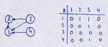
You can see that the element aij of matrix A is 1 if there is an edge from i to j, and the element is 0 if there is no edge from i to j (i is row, j is column). The storage space required by this representation is O(|V|2). For dense graphs this is ok, but for sparse it's not ok.
Adjacency list of a given vertex v ? V is the list Adj[v] of vertices adjacent to v. Here is an example of adjacency list for the same graph:
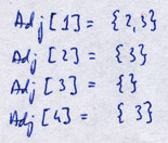
Storage required by this representation is O(V+E).
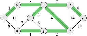
The lecture progresses with the problem of minimum spanning trees (MSTs). It's stated as following: given a connected, undirected graph G = (V, E) with edge weight function w: E -> R, find a spanning tree that connects all the vertices of minimum weight.
Here is an example of a MST. The MST of the graph is colored in green. The MST connects all the vertices of the graph so that the weight of edges is minimum.
Analyzing the MST problem in more detail, it is appears that MST contains optimal substructure property - if we take a subgraph and look at its MST, that MST will be a part of the MST of the whole graph. This is dynamic programming hallmark #1 (see previous lecture). It also appears that the problem of finding an MST contains overlapping subproblems, which is dynamic programming hallmark #2. Hallmarks #1 and #2 suggest that we could use a dynamic programming algorithm to find a MST of a graph. Surprisingly, there is something more powerful than dynamic programming algorithm for this problem - a greedy algorithm.
There is a hallmark for greedy algorithms:
- Greedy choice property - a locally optimal choice is globally optimal.
Lecture continues with a theorem and a proof that a greedy local choice for a MST is globally optimal choice. This is the key idea behind Prim's algorithm for finding a minimum spanning tree of a graph. The idea in the algorithm is to maintain a priority queue Q (keyed on minimum weight of edge connected to a vertex) of vertices that are not yet connected in the MST. At each step the algorithm takes a vertex from Q and goes over all edges, connects the edge with minimum weight to MST and updates keys of neighbor vertices (please see the lecture or lecture notes for the exact algorithm and an example).
The lecture ends with running time analysis of Prim's algorithm. As it uses a priority queue, the running time depends on implementation of the priority queue used. For example, if we use a dumb array as a priority queue, the running time is O(V2), if we use a binary heap, the running time os O(E·lg(V)), if we use a Fibonacci heap, the running time is O(E + V·lg(V)).
Another well known algorithm for MSTs is Kruskal's algorithm (runs in O(E·lg(V)), which uses a disjoint-set data structure, that is not covered in this course (but is covered in Chapter 21 of the book this course is taught from).
The best known algorithm to date for finding MSTs is by David R. Karger (MIT), Philip N. Klein (Brown University) and Robert E. Tarjan (Princeton University). This algorithm was found in 1993, it's randomized in nature and runs in O(E + V) expected time. Here is the publication that presents this algorithm: "A Randomized Linear-Time Algorithm for Finding Minimum Spanning Trees".
You're welcome to watch lecture sixteen:
Topics covered in lecture sixteen:
- [00:10] Review of graphs.
- [00:50] Digraph - directed graph.
- [01:50] Undirected graph.
- [02:40] Bound of edges in a graph |E| = O(V2).
- [04:10] Connected graph edges |E| >= |V| - 1.
- [05:50] Graph representations.
- [06:15] Adjacency matrix graph representation.
- [08:20] Example of adjacency matrix of a graph.
- [09:50] Storage required for an adjacency matrix O(V2). Dense representation.
- [12:40] Adjecency list graph representation.
- [13:40] Example of adjecancy list of a graph.
- [15:50] Handshaking lemma (theorem) for undirected graphs.
- [18:20] Storage required for adj. list representation O(E + V).
- [23:30] Minimum spanning trees.
- [24:20] Definition of MST problem.
- [28:45] Example of a graph and its minimum spanning tree.
- [34:50] Optimal substructure property of MST (dynamic programming hallmark #1).
- [38:10] Theorem that a subgraph's MST is part of whole graph's MST.
- [42:40] Cut and paste argument proof.
- [45:40] Overlapping subproblems of MST (dynamic programming hallmark #2).
- [48:20] Hallmark for greedy algorithms: The greedy choice property - a locally optimal choice is globally optimal.
- [50:25] Theorem and proof that a local choice of least weight edge is globally optimal for MSTs.
- [01:01:10] Prim's algorithm for minimum spanning trees.
- [01:01:50] Key idea of Prim's algorithm.
- [01:02:55] Pseudocode of Prim's algorithm.
- [01:07:40] Example of running Prim's algorithm.
- [01:15:03] Analysis of Prim's algorithm running time.
- [01:18:20] Running time if we choose array, binary heap and Fibonaci heap.
- [01:22:40] Kruskal's algorithm.
- [01:23:00] The best algorithm for MST to date.
Lecture sixteen notes:
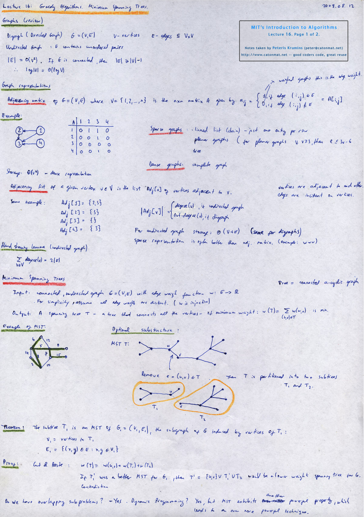 Lecture 16, page 1 of 2: graphs, graph representations, adjacency lists, minimum spanning trees, cut and paste argument.
|
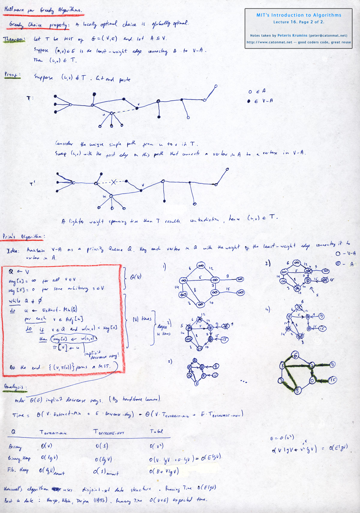 Lecture 16, page 2 of 2: greedy choice property, prim's algorithm, idea of kruskal's algorithm.
|
This course is taught from the Introduction to Algorithms book, also knows as CLRS book. Chapter 16 is titled Greedy Algorithms. It explains an activity-selection problem, elements of greedy algorithms, Huffman codes, Matroid theory, and task scheduling problem. Graphs are reviewed in Appendix B of the book.
The next post will be a trilogy of graph and shortest paths algorithms - Dijkstra's algorithm, Breadth-first search, Bellman-Ford algorithm, Floyd-Warshall algorithm and Johnson's algorithm.