 This is the second post in an article series about MIT's course Linear Algebra. In this post I will review lecture two on solving systems of linear equations by elimination and back-substitution. The other topics in the lecture are elimination matrices (also known as elementary matrices) and permutation matrices.
The first post covered the geometry of linear equations.
One of my blog readers, Seyed M. Mottaghinejad, had also watched this course and sent me his lecture notes. They are awesome. Grab them here: lecture notes by Seyed M. Mottaghinejad (includes .pdf, .tex and his document class).
Okay, here is the second lecture.
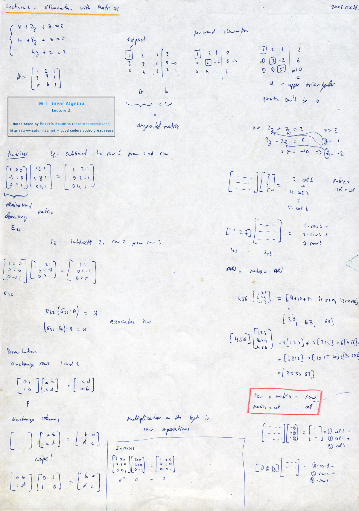
Lecture 2: Elimination with Matrices
Elimination is the way every software package solves equations. If the elimination succeeds it gets the answer. If the matrix A in Ax=b is a "good" matrix (we'll see what a good matrix is later) then the elimination will work and we'll get the answer in an efficient way. It's also always good to ask how can it fail. We'll see in this lecture how elimination decides if the matrix A is good or bad. After the elimination there is a step called back-substitution to complete the answer.
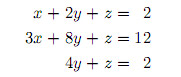
Okay, here is a system of equations. Three equations in three unknowns.
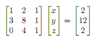
Remember from lecture one, that every such system can be written in the matrix form Ax=b, where A is the matrix of coefficients, x is a column vector of unknowns and b is the column vector of solutions (the right hand side). Therefore the matrix form of this example is the following:
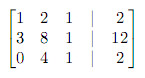
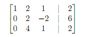
For the elimination process we need the matrix A and the column vector b. The idea is very simple, first we write them down in the augmented matrix form A|b:
Next we subtract rows from one another in such a way that the final result is an upper triangular matrix (a matrix with all the elements below the diagonal being zero).
So the first step is to subtract the first row multiplied by 3 from the second row. This gives us the following matrix:
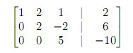
The next step is to subtract the second row multiplied by 2 from the third row. This is the final step and produces an upper triangular matrix that we needed:
Now let's write down the equations that resulted from the elimination:
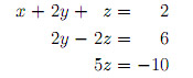
Working from the bottom up we can immediately find the solutions z, y, and x. From the last equation, z = -10/5 = -2. Now we put z in the middle equation and solve for y. 2y = 6 + 2z = 6 + 2(-2) = 6 - 4 = 2 => y = 1. And finally, we can substitute y and z in the first equation and solve for x. x = 2 - 2y - z = 2 - 2(1) - (-2) = 2.
We have found the solution, it's (x=2, y=1, z=-2). The process we used to find it is called the back-substitution.
The elimination would fail if taking a multiple of one row and adding to the next would produce a zero on the diagonal (and there would be no other row to try to exchange the failing row with).
The lecture continues with figuring out how to do the elimination by using matrices. In the first lecture we learned that a matrix times a column vector gave us a combination of the columns of the matrix. Similarly, a row times a matrix gives us a combination of the rows of the matrix.
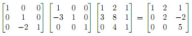
Let's look at our first step of elimination again. It was to subtract 3 times the first row from the second row. This can be expressed as matrix multiplication (forget the column b for a while):
Let's call the matrix on the right E as elimination matrix (or elementary matrix), and give it subscript E21 for making a zero in the resulting matrix at row 2, column 1.
The next step was twice the second row minus the third row:
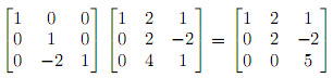
The matrix on the right is again an elimination matrix. Let's call it E32 for giving a zero at row 3, column 2.
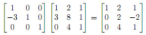
But notice that these two operations can be combined:
And we can write E32(E21A) = U. Now remember that matrix operations are associative, therefore we can change the parenthesis (E32E21)A = U. If we multiply (E32E21) we get a single matrix E that we will call the elimination matrix. What we have done is expressed the whole elimination process in matrix language!
Next, the lecture continues takes a step back and looks at permutation matrices. The question asked is "what matrix would exchange two rows of a matrix?" and "what matrix would exchange two columns of a matrix?"
Watch the lecture to find the answer to these questions!
Topics covered in lecture two:
- [00:25] Main topic for today: elimination.
- [02:35] A system with three equations and three unknowns:
- [03:30] Elimination process. Taking matrix A to U.
- [08:35] Three pivots of matrix U.
- [10:15] Relation of pivots to determinant of a matrix.
- [10:40] How can elimination fail?
- [14:40] Back substitution. Solution (x=2, y=1, z=-2).
- [19:45] Elimination with matrices.
- [21:10] Matrix times a column vector is a linear combination of columns the matrix.
- [22:15] A row vector times a matrix is a linear combination of rows of the matrix.
- [23:40] Matrix x column = column.
- [24:10] Row x matrix = row.
- [24:20] Elimination matrix for subtracting three times row one from row two.
- [26:55] The identity matrix.
- [30:00] Elimination matrix for subtracting two times row two from row three.
- [32:40] E32E21A = U.
- [37:20] Permutation matrices.
- [37:30] How to exchange rows of a 2x2 matrix?
- [37:55] Permutation matrix P to exchange rows of a 2x2 matrix.
- [38:40] How to exchange columns of a 2x2 matrix?
- [39:40] Permutation matrix P to exchange columns of a 2x2 matrix.
- [42:00] Commutative law does not hold for matrices.
- [44:25] Introduction to inverse matrices.
- [47:10] E-1E = I.
Here are my notes of lecture two:
 My notes of linear algebra lecture 2 on elimination with matrices.
The next post is going to be either on lectures three and four together or just lecture three. Lecture three will touch a bit more on matrix multiplication and then dive into the inverse matrices. Lecture four will cover A=LU matrix decomposition (also called factorization).