 This is the third post in an article series about MIT's Linear Algebra course. In this post I will review lecture three on five ways to multiply matrices, inverse matrices and an algorithm for finding inverse matrices called Gauss-Jordan elimination.
The first lecture covered the geometry of linear equations and the second lecture covered the matrix elimination.
Here is lecture three.
Lecture 3: Matrix Multiplication and Inverse Matrices
Lecture three starts with five ways to multiply matrices.
The first way is the classical way. Suppose we are given a matrix A of size mxn with elements aij and a matrix B of size nxp with elements bjk, and we want to find the product A·B. Multiplying matrices A and B will produce matrix C of size mxp with elements  .
.
Here is how this sum works. To find the first element c11 of matrix C, we sum over the 1st row of A and the 1st column of B. The sum expands to c11 = a11·b11 + a12·b21 + a13·b31 + ... + a1n·bn1. Here is a visualization of the summation:
We continue this way until we find all the elements of matrix C. Here is another visualization of finding c23:
The second way is to take each column in B, multiply it by the whole matrix A and put the resulting column in the matrix C. The columns of C are combinations of columns of A. (Remember from previous lecture that a matrix times a column is a column.)
For example, to get column 1 of matrix C, we multiply A·(column 1 of matrix B):
The third way is to take each row in A, multiply it by the whole matrix B and put the resulting row in the matrix C. The rows of C are combinations of rows of B. (Again, remember from previous lecture that a row times a matrix is a row.)
For example, to get row 1 of matrix C, we multiply row 1 of matrix A with the whole matrix B:
The fourth way is to look at the product of A·B as a sum of (columns of A) times (rows of B).
Here is an example:
The fifth way is to chop matrices in blocks and multiply blocks by any of the previous methods.
Here is an example. Matrix A gets subdivided in four submatrices A1 A2 A3 A4, matrix B gets divided in four submatrices B1 B2 B3 B4 and the blocks get treated like simple matrix elements.
Here is the visualization:
Element C1, for example, is obtained by multiplying A1·B1 + A2·B3.
Next the lecture proceeds to finding the inverse matrices. An inverse of a matrix A is another matrix, such that A-1·A = I, where I is the identity matrix. In fact if A-1 is the inverse matrix of a square matrix A, then it's both the left-inverse and the right inverse, i.e., A-1·A = A·A-1 = I.
If a matrix A has an inverse then it is said to be invertible or non-singular.
Matrix A is singular if we can find a non-zero vector x such that A·x = 0. The proof is easy. Suppose A is not singular, i.e., there exists matrix A-1. Then A-1·A·x = 0·A-1, which leads to a false statement that x = 0. Therefore A must be singular.
Another way of saying that matrix A is singular is to say that columns of matrix A are linearly dependent (one ore more columns can be expressed as a linear combination of others).
Finally, the lecture shows a deterministic method for finding the inverse matrix. This method is called the Gauss-Jordan elimination. In short, Gauss-Jordan elimination transforms augmented matrix (A|I) into (I|A-1) by using only row eliminations.
Please watch the lecture to find out how it works in all the details:
Topics covered in lecture three:
- [00:51] The first way to multiply matrices.
- [04:50] When are we allowed to multiply matrices?
- [06:45] The second way to multiply matrices.
- [10:10] The third way to multiply matrices.
- [12:30] What is the result of multiplying a column of A and a row of B?
- [15:30] The fourth way to multiply matrices.
- [18:35] The fifth way to multiply matrices by blocks.
- [21:30] Inverses for square matrices.
- [24:55] Singular matrices (no inverse matrix exists).
- [30:00] Why singular matrices can't have inverse?
- [36:20] Gauss-Jordan elimination.
- [41:20] Gauss-Jordan idea A·I -> I·A-1.
Here are my notes of lecture three:
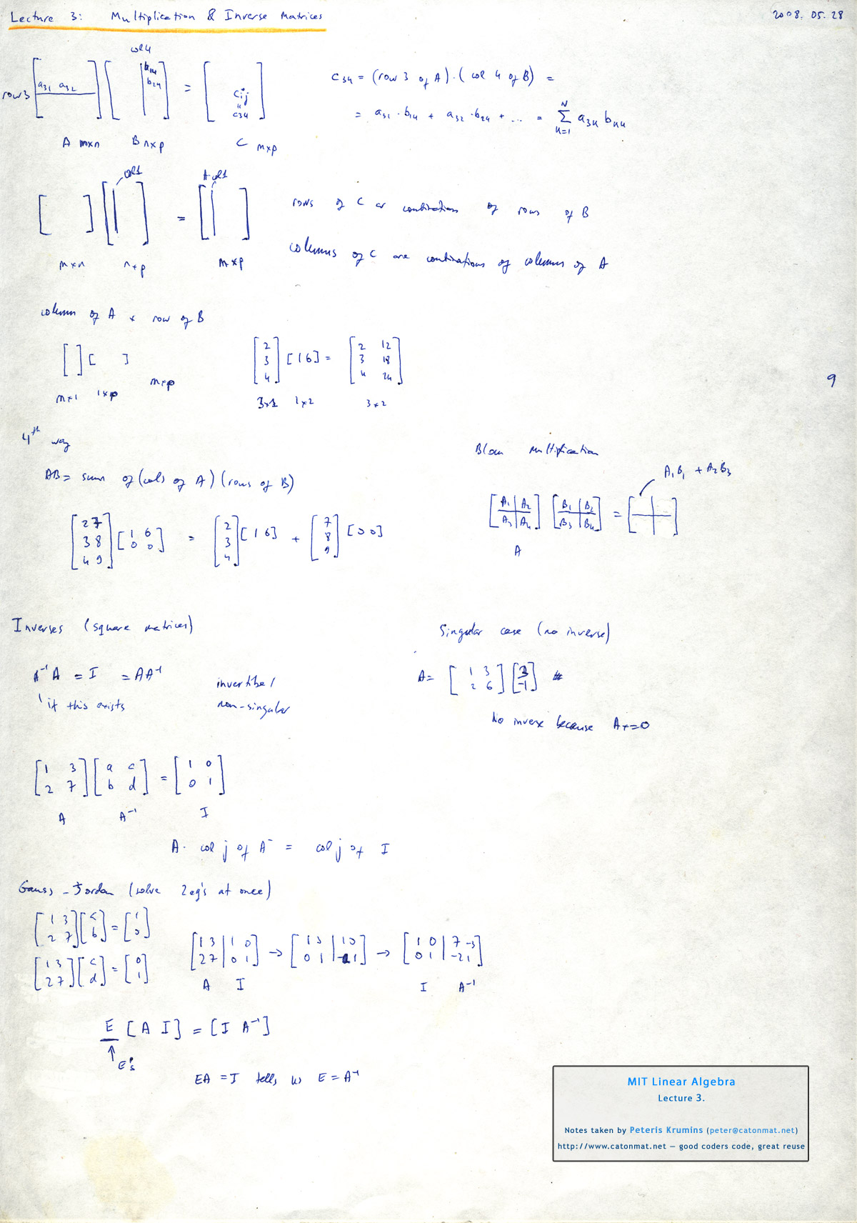 My notes of linear algebra lecture 3 on the matrix multiplication and inverses.
The next post is going to be about the A=LU matrix decomposition (also known as factorization).