MIT’s Introduction to Algorithms, Lectures 4 and 5: Sorting

This is the third post in an article series about MIT’s lecture course “Introduction to Algorithms.” In this post I will review lectures four and five, which are on the topic of sorting.

The previous post covered a lecture on “Divide and Conquer” algorithm design technique and its applications.

Lecture four is devoted entirely to a single sorting algorithm which uses this technique. The algorithm I am talking about is the “Quicksort” algorithm. The quicksort algorithm was invented by Charles Hoare in 1962 and it is the most widely used sorting algorithm in practice.

I wrote about quicksort before in “Three Beautiful Quicksorts” post, where its running time was analyzed experimentally. This lecture does it theoretically.

Lecture five talks about theoretical running time limits of sorting using comparisons and then discusses two linear time sorting algorithms — Counting sort and Radix sort.

Lecture 4: Quicksort

The lecture starts by giving the divide and conquer description of the algorithm:

• Divide: Partition the array to be sorted into two subarrays around pivot x, such that elements in the lower subarray <= x, and elements in the upper subarray >= x.
• Conquer: Recursively sort lower and upper subarrays using quicksort.
• Combine: Since the subarrays are sorted in place, no work is needed to combine them. The entire array is now sorted!

The main algorithm can be written in a few lines of code:

Quicksort(A, p, r) // sorts list A[p..r]
  if p < r
    q = Partition(A, p, r)
    Quicksort(A, p, q-1)
    Quicksort(A, q+1, r)

The key in this algorithm is the Partition subroutine:

Partition(A, p, q)
  // partitions elements in array A[p..q] in-place around element x = A[p],
  // so that A[p..i] <= x and A[i] == x and A[i+1..q] >= x
  x = A[p]
  i = p
  for j = p+1 to q
    if A[j] <= x
      i = i+1
      swap(A[i], A[j])
  swap(A[p], A[i])
  return i

The lecture then proceeds with the analysis of Quicksort’s worst-case running time. It is concluded that if the array to be sorted is already sorted or already reverse sorted, the running time is O(n²), which is no better than Insertion sort (seen in lecture one)! What happens in the worst case is that all the elements get partitioned to one side of the chosen pivot. For example, given an array (1, 2, 3, 4), the partition algorithm chooses 1 as the pivot, then all the elements stay where they were, and no partitioning actually happens. To overcome this problem Randomized Quicksort algorithm is introduced.

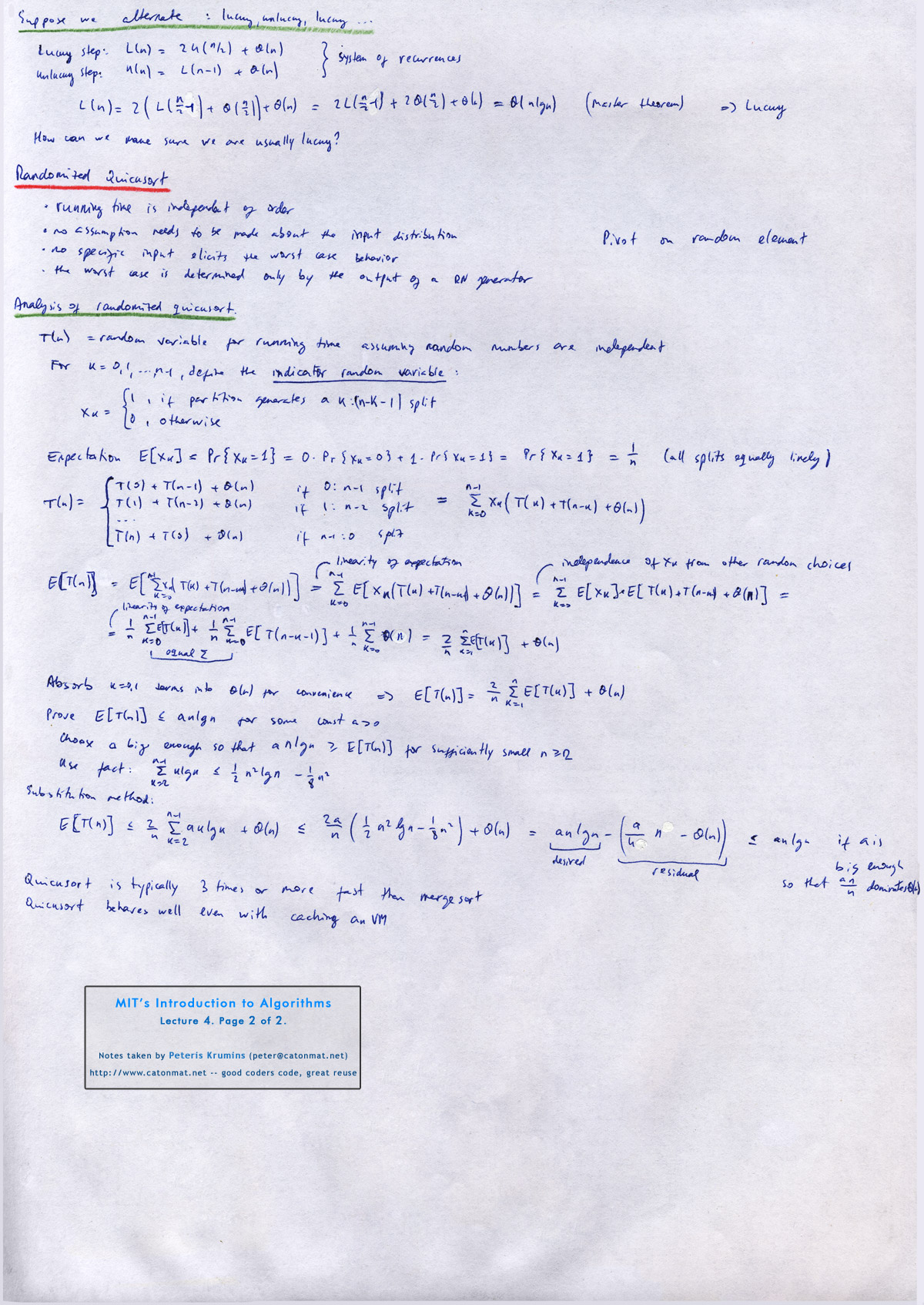
The main idea of randomized quicksort hides in the Partition subroutine. Instead of partitioning around the first element, it partition around a random element in the array!

Nice things about randomized quicksort are:

• Its running time is independent of initial element order.
• No assumptions need to be made about the statistical distribution of input.
• No specific input elicits the worst case behavior.
• The worst case is determined only by the output of a random-number generator.

Randomized-Partition(A, p, q)
  swap(A[p], A[rand(p,q)]) // the only thing changed in the original Partition subroutine!
  x = A[p]
  i = p
  for j = p+1 to q
    if A[j] <= x
      i = i+1
      swap(A[i], A[j])
  swap(A[p], A[i])
  return i

The rest of the lecture is very math-heavy and uses indicator random variables to conclude that the expected running time of randomized quicksort is O(n·lg(n)).

In practice quicksort is 3 or more times faster than merge sort.

Please see Three Beautiful Quicksorts post for more information about the version of industrial-strength quicksort.

You’re welcome to watch lecture four:

Topics covered in lecture four:

• [00:35] Introduction to quicksort.
• [02:30] Divide and conquer approach to quicksort.
• [05:20] Key idea - linear time (Θ(n)) partitioning subroutine.
• [07:50] Structure of partitioning algorithm.
• [11:40] Example of partition algorithm run on array (6, 10, 13, 5, 8, 3, 2, 11).
• [16:00] Pseudocode of quicksort algorithm.
• [19:00] Analysis of quicksort algorithm.
• [20:25] Worst case analysis of quicksort.
• [24:15] Recursion tree for worst case.
• [28:55] Best case analysis of quicksort, if partition splits elements in half.
• [28:55] Analysis of quicksort, if partition splits elements in a proportion 1/10 : 9/10.
• [33:33] Recursion tree of this analysis.
• [04:30] Analysis of quicksort, if partition alternates between lucky, unlucky, lucky, unlucky, …
• [46:50] Randomized quicksort.
• [51:10] Analysis of randomized quicksort.

Lecture four notes:

Lecture 4, page 1 of 2.

Lecture 4, page 2 of 2.

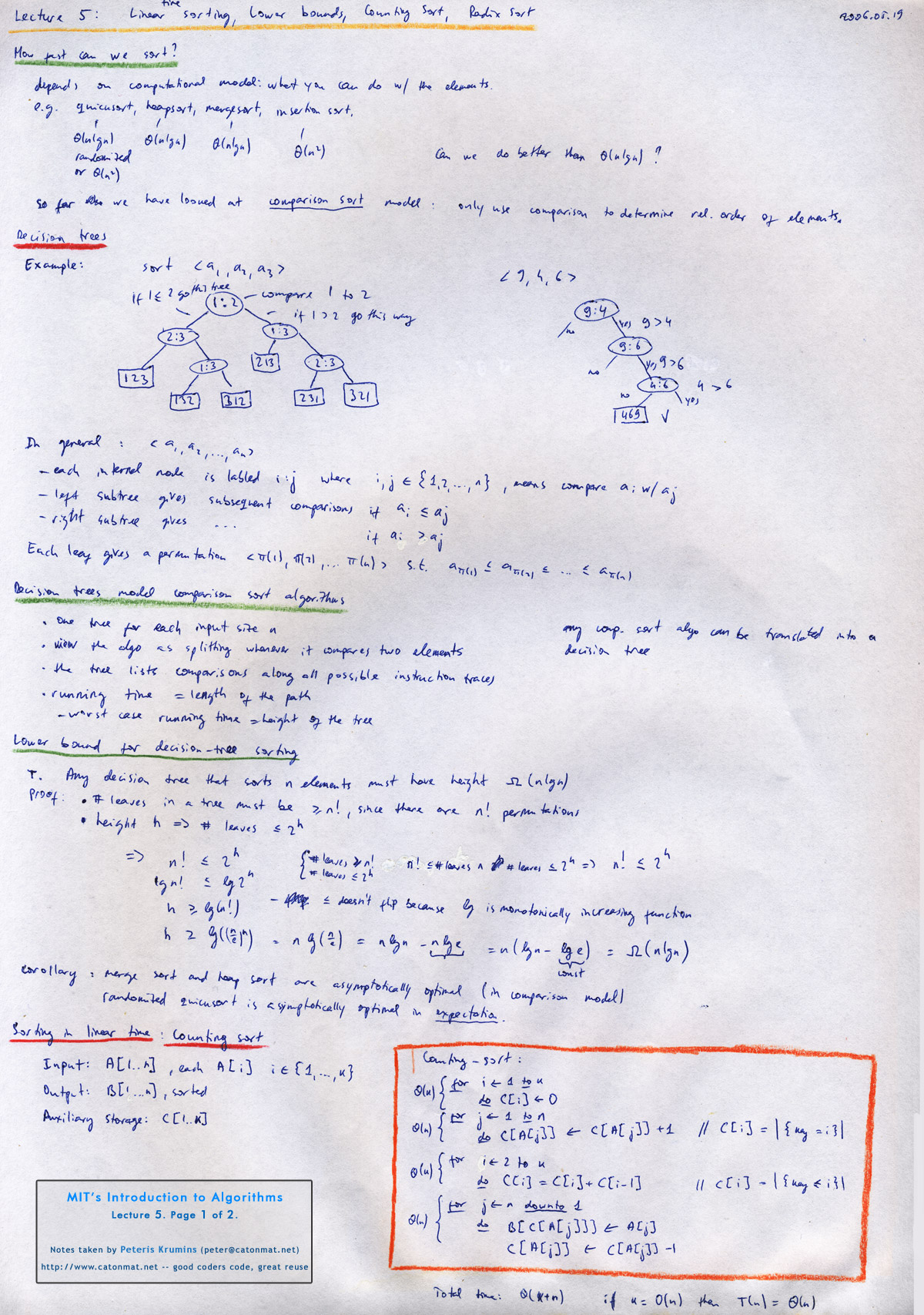
Lecture 5: Lower Sorting Bounds and Linear Sorting

The lecture starts with a question — How fast can we sort? Erik Demaine (professor) answers and says that it depends on the model of what you can do with the elements.

The previous lectures introduced several algorithms that can sort n numbers in O(n·lg(n)) time. Merge sort achieves this upper bound in the worst case; quicksort achieves it on average. These algorithms share an interesting property: the sorted order they determine is based only on comparisons between the input elements. Such sorting algorithms are called Comparison Sorts, which is a model for sorting.

It turns out that any comparison sort algorithm can be translated into something that is called a Decision Tree. A decision tree is a full binary tree that represents the comparisons between elements that are performed by a particular sorting algorithm operating on an input of a given size.

Erik uses decision trees to derive the lower bound for running time of comparison based sorting algorithms. The result is that no comparison-based sort can do better than O(n·lg(n)).

The lecture continues with bursting outside of comparison model and looks at sorting in linear time using no comparisons.

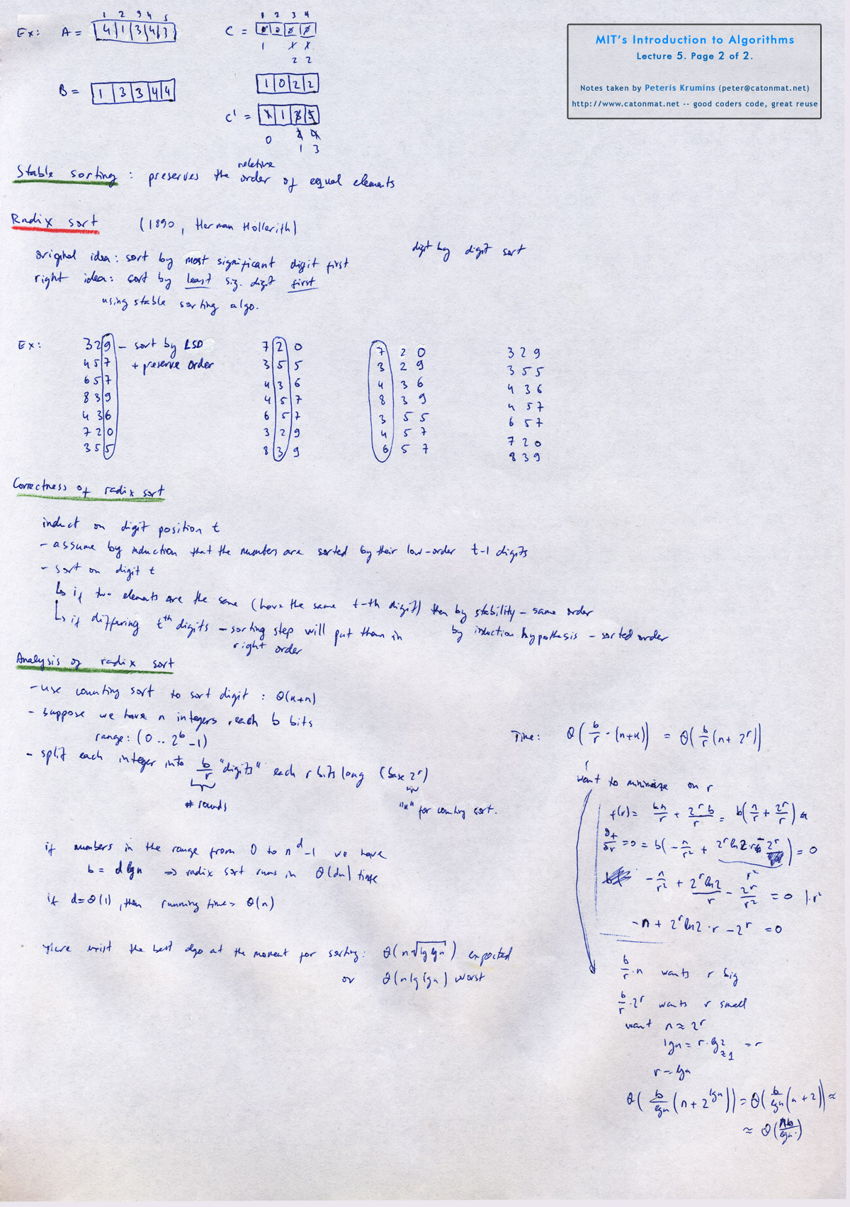
The first linear time algorithm covered in the lecture is Counting Sort. The basic idea of counting sort is to determine, for each input element x, the number of elements less than x. This information can be used to place element x directly into its position in the output array. For example, if there are 17 elements less than x, then x belongs in output position 18.

The second linear time algorithm is Radix Sort, which sorts a list of numbers by examining each digit at a given position separately.

Erik ends the lecture by analyzing correctness and running time of radix sort.

Video of lecture five:

Topics covered in lecture five:

• [00:30] How fast can we sort?
• [02:27] Review of running times of quicksort, heapsort, merge sort and insertion sort.
• [04:50] Comparison sorting (model for sorting).
• [06:50] Decision trees.
• [09:35] General description of decision trees.
• [14:25] Decision trees model comparison sorts.
• [20:00] Lower bound on decision tree sorting.
• [31:35] Sorting in linear time.
• [32:30] Counting sort.
• [38:05] Example of counting sort run on an array (4, 1, 3, 4, 3)
• [50:00] Radix sort.
• [56:10] Example of radix sort run on array (329, 457, 657, 839, 546, 720, 355).
• [01:00:30] Correctness of radix sort.
• [01:04:25] Analysis of radix sort.

Lecture five notes:

Lecture 5, page 1 of 2.

Lecture 5, page 2 of 2.

Have fun sorting! The next post will be about order statistics (given an array find n-th smallest element)!

PS. This course is taught from the CLRS book (also called “Introduction to Algorithms”):