![]() This is the sixth post in an article series about MIT's lecture course "Introduction to Algorithms." In this post I will review lectures nine and ten, which are on the topic of Search Trees.
This is the sixth post in an article series about MIT's lecture course "Introduction to Algorithms." In this post I will review lectures nine and ten, which are on the topic of Search Trees.
Search tree data structures provide many dynamic-set operations such as search, insert, delete, minimum element, maximum element and others. The complexity of these operations is proportional to the height of the tree. The better we can balance the tree, the faster they will be. Lectures nine and ten discuss two such structures.
Lecture nine discusses randomly built binary search trees. A randomly built binary search tree is a binary tree that arises from inserting the keys in random order into an initially empty tree. The key result shown in this lecture is that the height of this tree is O(lg(n)).
Lecture ten discusses red-black trees. A red-black tree is a binary search tree with extra bit of information at each node -- it's color, which can be either red or black. By contrasting the way nodes are colored on any path from the root to a leaf, red-black trees ensure that the tree is balanced, giving us guarantees that the operations on this tree will run on O(lg(n)) time!
PS. Sorry for being silent for the past two weeks. I am preparing for job interviews at a company starting with 'G' and it is taking all my time. ;)
Lecture 9: Randomly Built Binary Search Trees
Lecture nine starts with an example of good and bad binary search tree. Given a binary tree with n nodes, a good trees has height log(n) but the bad one has height close to n. As the basic operations on trees run in time proportional to the height of the tree, it's recommended that we build the good trees and not the bad ones.
Before discussing randomly built binary search trees, professor Erik Demaine shows another sorting algorithm. It's called binary search tree sort (BST-sort). It's amazingly simple -- given an array of n items to sort, build a BST out of it and do an in-order tree walk on it. In-order tree walk walks the left branch first, then prints the values, and then walks the right branch. Can you see why the printed list of values is sorted? (If not see the lecture ;) ) [part three of the article series covers sorting algorithms]
Turns out that there is a relation between BST-sort and quicksort algorithm. BST-sort and quicksort make the same comparisons but in different order. [more info on quicksort in part two of article series and in "three beautiful quicksorts" post]
After this discussion, the lecture finally continues with randomized BST-sort which leads to idea of randomly built BSTs.
The other half of the lecture is devoted to a complicated proof of the expected height of a randomly built binary search tree. The result of this proof is that the expected height is order log(n).
You're welcome to watch lecture nine:
Topics covered in lecture nine:
- [00:50] Good and bad binary search trees (BSTs).
- [02:00] Binary search tree sort tree algorithm.
- [03:45] Example of running BST-sort on array (3, 1, 8, 2, 6, 7, 5).
- [05:45] Running time analysis of BST-sort algorithm.
- [11:45] BST-sort relation to quicksort algorithm.
- [16:05] Randomized BST-sort.
- [19:00] Randomly built binary search trees.
- [24:58] Theorem: expected height of a rand BST tree is O(lg(n)).
- [26:45] Proof outline.
- [32:45] Definition of convex function.
- [46:55] Jensen's inequality.
- [55:55] Expected random BST height analysis.
Lecture nine notes:
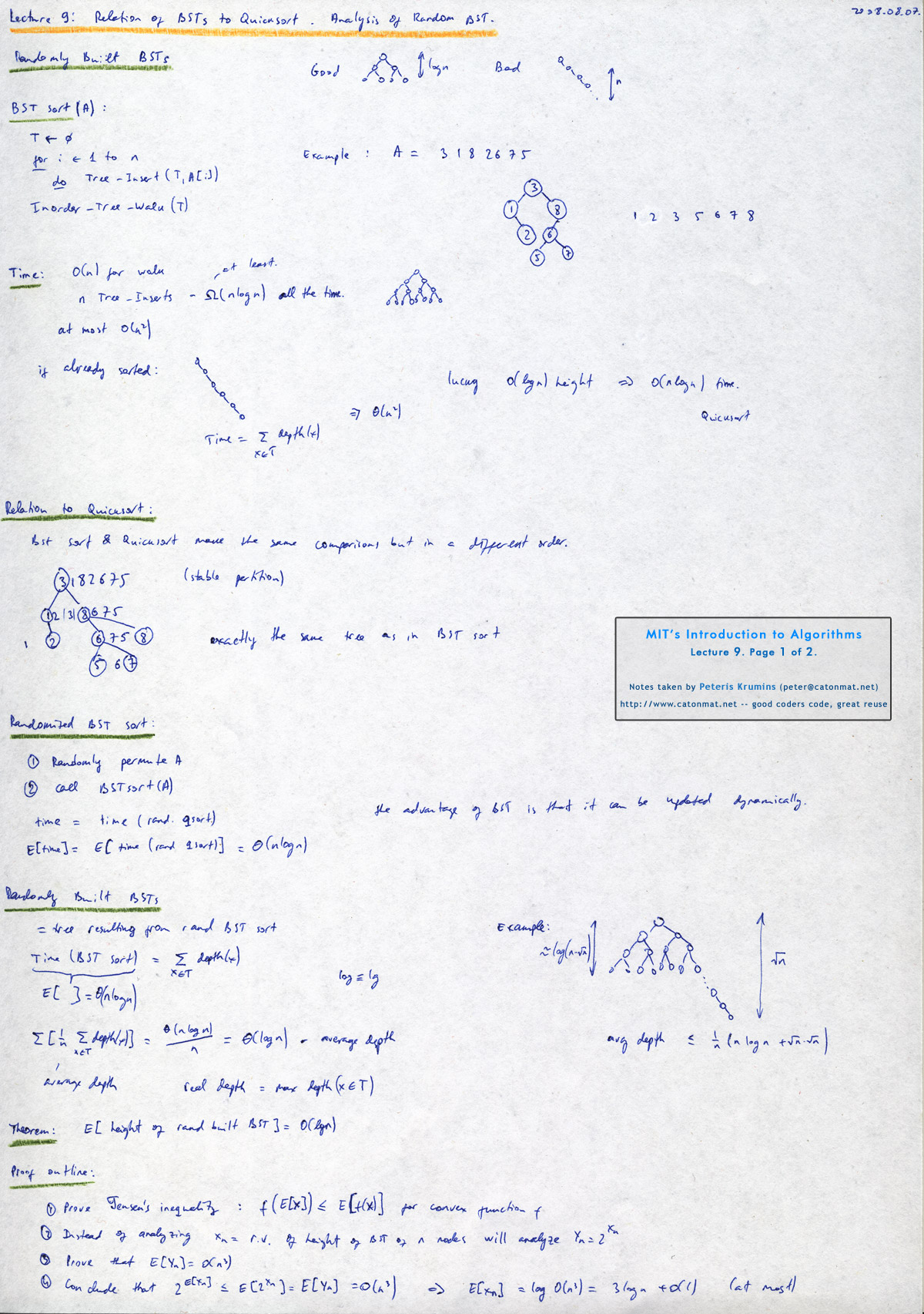 Lecture 9, page 1 of 2.
|
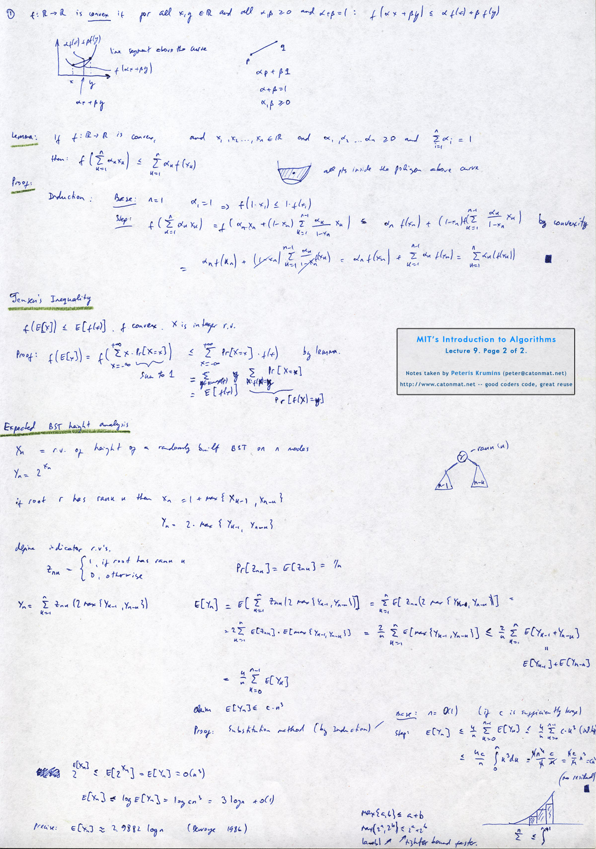 Lecture 9, page 2 of 2.
|
Lecture 10: Red-Black Trees
Lecture ten begins with a discussion of balanced search trees. Balanced search tree is search tree data structure maintain a dynamic set of n elements using tree of height log(n).
There are many balanced search tree data structures. For example: AVL trees (invented in 1964), 2-3 trees (invented in 1970), 2-3-4 trees, B-trees, red-black trees, skiplists, treaps.
This lecture focuses exclusively on red-black trees.
Red-black trees are binary search trees with extra color field for each node. They satisfy red-black properties:
- Every node is either red or black.
- The root and leaves are black.
- Every red node has a black parent.
- All simple paths from a node to x to a descendant leaf of x have same number of black nodes = black-height(x).
The lecture gives a proof sketch of the height of an RB-tree and discusses running time of queries (search, min, max, successor, predecessor operations) and then goes into details of update operations (insert, delete). Along the way rotations on a tree are defined, the right-rotate and left-rotate ops.
The other half of the lecture looks at Red-Black-Insert operation that inserts an element in the tree while maintaining the red-black properties.
Here is the video of lecture ten:
Topics covered in lecture ten:
- [00:35] Balanced search trees.
- [02:30] Examples of balanced search tree data structures.
- [05:16] Red-black trees.
- [06:11] Red-black properties.
- [11:26] Example of red-black tree.
- [17:30] Height of red-black tree.
- [18:50] Proof sketch of RBtree height.
- [21:30] Connection of red-black trees to 2-3-4 trees.
- [32:10] Running time of query operations.
- [35:37] How to do RB-tree updates (inserts, deletes)?
- [36:30] Tree rotations.
- [40:55] Idea of red-black tree insert operation.
- [44:30] Example of inserting an element in a tree.
- [54:30] RB-Insert algorithm.
- [01:03:35] The three cases in insert operation.
Lecture ten notes:
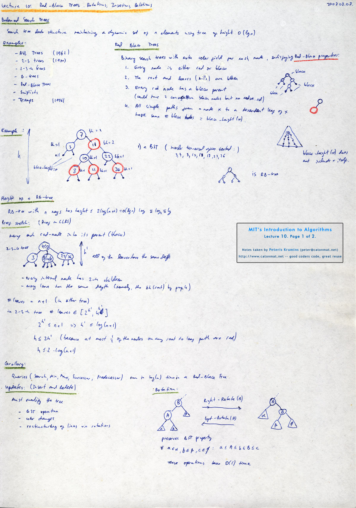 Lecture 10, page 1 of 2.
|
 Lecture 10, page 2 of 2.
|
Have fun building trees! The next post will be about general methodology of augmenting data structures and it will discuss dynamic order statistics and interval trees.