![]() This is the ninth post in an article series about MIT's lecture course "Introduction to Algorithms." In this post I will review lectures thirteen and fourteen. They are on theoretical topics of Amortized Analysis, Competitive Analysis and Self-Organizing Lists.
This is the ninth post in an article series about MIT's lecture course "Introduction to Algorithms." In this post I will review lectures thirteen and fourteen. They are on theoretical topics of Amortized Analysis, Competitive Analysis and Self-Organizing Lists.
Amortized analysis is a tool for analyzing algorithms that perform a sequence of similar operations. It can be used to show that the average cost of an operation is small, if one averages over a sequence of operations, even though a single operation within the sequence might be expensive. Amortized analysis differs from average-case analysis in that probability is not involved; an amortized analysis guarantees the average performance of each operation in the worst case.
Lecture thirteen looks at three most common techniques used in amortized analysis - Aggregate Analysis, Accounting Method (also known as Taxation Method) and Potential Method.
Competitive analysis is a method that is used to show how an Online Algorithm compares to an Offline Algorithm. An algorithm is said to be online if it does not know the data it will be executing on beforehand. An offline algorithm may see all of the data in advance.
A self-organizing list is a list that reorders its elements based on some self-organizing heuristic to improve average access time.
Lecture fourteen gives a precise definition of what it means for an algorithm to be competitive and shows a heuristic for a self-organizing list that makes it 4-competitive.
Lecture 13: Amortized Algorithms
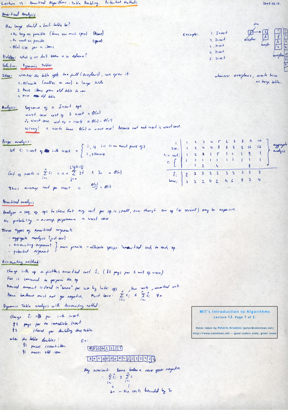
Lecture thirteen starts with a question - "How large should a hash table be?" Well, we could make it as large as possible to minimize the search time, but then it might take too much space. We could then try to make it as small as possible, but what if we don't know the number of elements that will be hashed into it? The solution is to use a dynamic hash table that grows whenever it is about to overflow.
This creates a problem that at the moment of overflow the table must be grown and growing it might take a lot of time. Thus, we need a way to analyze the running time in a long run.
Lecture continues with three methods for this analysis, called amortized arguments - aggregate method, accounting method, and potential method.
In aggregate analysis, we determine an upper bound T(n) on the total cost of a sequence of n operations. The average cost per operation is then T(n)/n. We take the average cost as the amortized cost of each operation, so that all operations have the same amortized cost.
In accounting method we determine an amortized cost of each operation. When there is more than one type of operation, each type of operation may have a different amortized cost. The accounting method overcharges some operations early in the sequence, storing the overcharge as "prepaid credit" on specific objects in the data structure. The credit is used later in the sequence to pay for operations that are charged less than they actually cost.
Potential method is like the accounting method in that we determine the amortized cost of each operation and may overcharge operations early on to compensate for undercharges later. The potential method maintains the credit as the "potential energy" of the data structure as a whole instead of associating the credit with individual objects within the data structure.
Each method is applied to dynamic tables to show that average cost per insert is O(1).
You're welcome to watch lecture thirteen:
Topics covered in lecture thirteen:
- [01:05] How large should a hash table be?
- [04:45] Dynamic tables.
- [06:15] Algorithm of dynamic hash tables.
- [07:10] Example of inserting elements in a dynamic array.
- [09:35] Wrong analysis of time needed for n insert operations.
- [12:15] Correct analysis of n insert operations using aggregate analysis method.
- [19:10] Definition of amortized analysis.
- [21:20] Types of amortized arguments.
- [23:55] Accounting method (taxation method) amortized analysis.
- [29:00] Dynamic table analysis with accounting (taxation) method.
- [40:45] Potential method amortized analysis.
- [54:15] Table doubling analysis with potential method.
- [01:13:10] Conclusions about amortized costs, methods and bounds.
Lecture thirteen notes:
 Lecture 13, page 1 of 2.
|
 Lecture 13, page 2 of 2.
|
Lecture 14: Competitive Analysis and Self-Organizing Lists
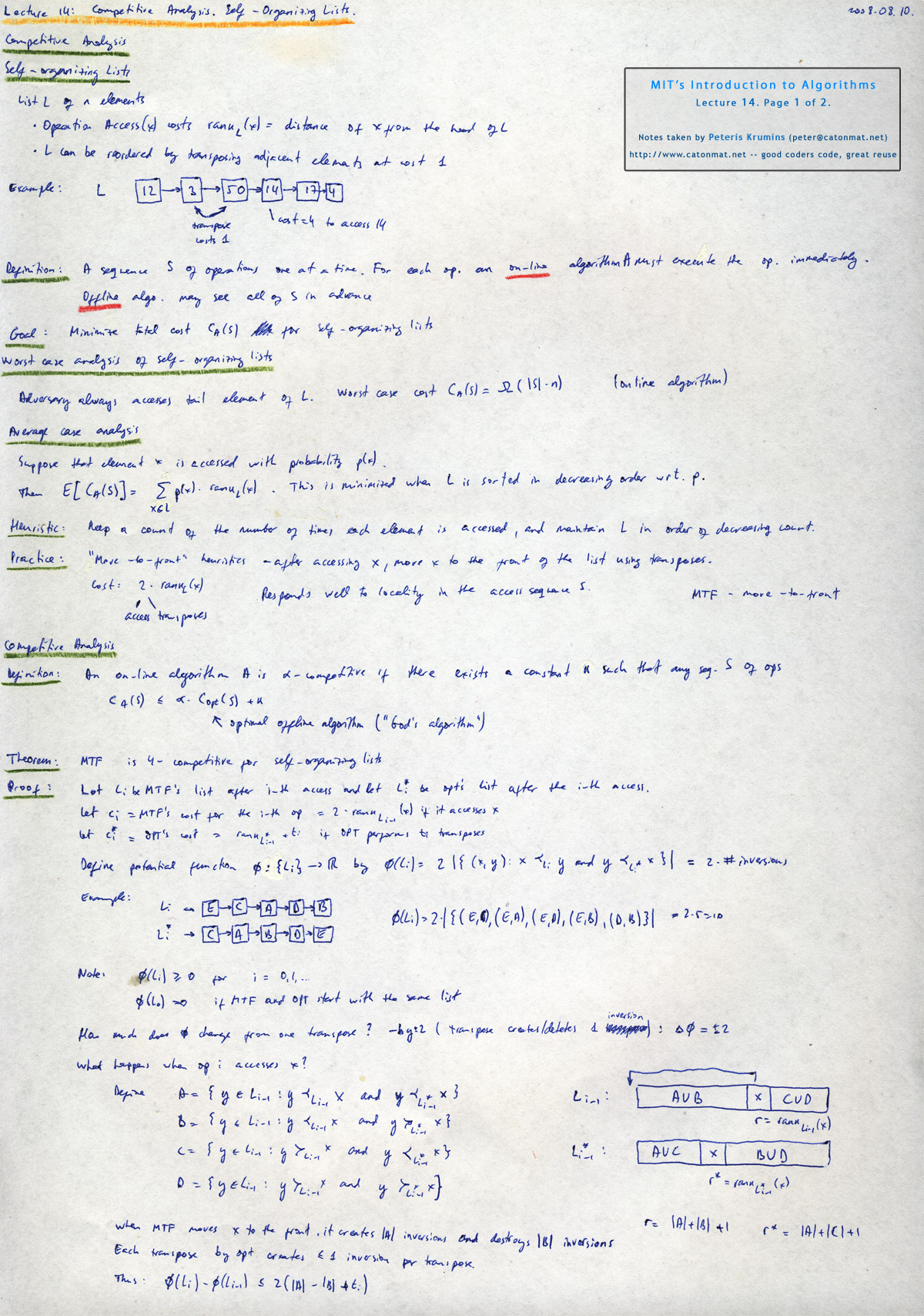
Lecture fourteen starts with the notion of self-organizing lists. A self-organizing list is a list that reorders itself to improve the average access time. The goal is to find a reordering that minimizes the total access time.
At this point the lecture steps away from this problem for a moment and defines online algorithms and offline algorithms: Given a sequence S of operations that algorithm must execute, an online algorithm must execute each operation immediately but an offline algorithm may see all of S in advance.
Now the lecture returns to the self-organizing list problem and looks at two heuristics how the list might reorganize itself to minimize the access time. The first way is to keep a count of the number of times each element in the list is accessed and reorder list in the order of decreasing count. The other is move-to-front heuristic (MTF) - after accessing the element, move it to the front of the list.
Next the lecture defines what it means for an algorithm to be competitive. It is said that an online algorithm is ?-competitive if there is a constant k such that for any sequence of operations the (running time cost of online algorithm) <= ?·(running time cost of an optimal offline algorithm (also called "God's algorithm")) + k.
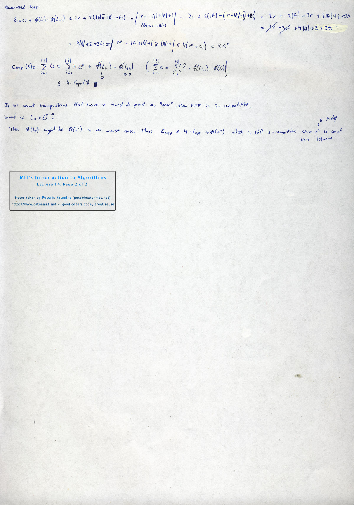
Lecture continues with a theorem that move-to-front is 4-competitive for self-organizing lists. The proof of this theorem takes almost an hour!
Topics covered in lecture fourteen:
- [01:00] Definition of self-organizing lists.
- [03:00] Example of a self-organizing list (illustrates transpose cost and access cost).
- [05:00] Definition of on-line and off-line algorithms.
- [08:45] Worst case analysis of self-organizing lists.
- [11:40] Average case analysis of selforganizing lists.
- [17:05] Move-to-front heuristic.
- [20:35] Definition of competitive analysis.
- [23:35] Theorem: MTF is 4-competitive.
- [25:50] Proof of this theorem.
Lecture fourteen notes:
 Lecture 14, page 1 of 2.
|
 Lecture 14, page 2 of 2.
|
Have fun with amortized and competitive analysis! The next post will be about dynamic programming.