![]() This is the twelfth post in an article series about MIT's lecture course "Introduction to Algorithms." In this post I will review a trilogy of lectures on graph and shortest path algorithms. They are lectures seventeen, eighteen and nineteen. They'll cover Dijkstra's Algorithm, Breadth-First Search Algorithm and Bellman-Ford Algorithm for finding single-source shortest paths as well as Floyd-Warshall Algorithm and Johnson's Algorithm for finding all-pairs shortest paths.
This is the twelfth post in an article series about MIT's lecture course "Introduction to Algorithms." In this post I will review a trilogy of lectures on graph and shortest path algorithms. They are lectures seventeen, eighteen and nineteen. They'll cover Dijkstra's Algorithm, Breadth-First Search Algorithm and Bellman-Ford Algorithm for finding single-source shortest paths as well as Floyd-Warshall Algorithm and Johnson's Algorithm for finding all-pairs shortest paths.
These algorithms require a thorough understanding of graphs. See the previous lecture for a good review of graphs.
Lecture seventeen focuses on the single-source shortest-paths problem: Given a graph G = (V, E), we want to find a shortest path from a given source vertex s ? V to each vertex v ? V. In this lecture the weights of edges are restricted to be positive which leads it to Dijkstra's algorithm and in a special case when all edges have unit weight to Breadth-first search algorithm.
Lecture eighteen also focuses on the same single-source shortest-paths problem, but allows edges to be negative. In this case a negative-weight cycles may exist and Dijkstra's algorithm would no longer work and would produce incorrect results. Bellman-Ford algorithm therefore is introduced that runs slower than Dijkstra's but detects negative cycles. As a corollary it is shown that Bellman-Ford solves Linear Programming problems with constraints in form xj - xi <= wij.
Lecture nineteen focuses on the all-pairs shortest-paths problem: Find a shortest path from u to v for every pair of vertices u and v. Although this problem can be solved by running a single-source algorithm once from each vertex, it can be solved faster with Floyd-Warshall algorithm or Johnson's algorithm.
Lecture 17: Shortest Paths I: Single-Source Shortest Paths and Dijkstra's Algorithm
Lecture seventeen starts with a small review of paths and shortest paths.
It reminds that given a graph G = (V, E, w), where V is a set of vertices, E is a set of edges and w is weight function that maps edges to real-valued weights, a path p from a vertex u to a vertex v in this graph is a sequence of vertices (v0, v1, ..., vk) such that u = v0, v = vk and (vi-1, vi) ? E. The weight w(p) of this path is a sum of weights over all edges = w(v0, v1) + w(v1, v2) + ... + w(vk-1, vk). It also reminds that a shortest path from u to v is the path with minimum weight of all paths from u to v, and that a shortest path in a graph might not exist if it contains a negative weight cycle.
The lecture then notes that shortest paths exhibit the optimal substructure property - a subpath of a shortest path is also a shortest path. The proof of this property is given by cut and paste argument. If you remember from previous two lectures on dynamic programming and greedy algorithms, an optimal substructure property suggests that these two techniques could be applied to solve the problem efficiently. Indeed, applying the greedy idea, Dijkstra's algorithm emerges.
Here is a somewhat precise definition of single-source shortest paths problem with non-negative edge weights: Given a graph G = (V, E), and a starting vertex s ? V, find shortest-path weights for all vertices v ? V.
Here is the greedy idea of Dijkstra's algorithm:
- 1. Maintain a set S of vertices whose shortest-path from s are known (s ? S initially).
- 2. At each step add vertex v from the set V-S to the set S. Choose v that has minimal distance from s (be greedy).
- 3. Update the distance estimates of vertices adjacent to v.
I have also posted a video interview with Edsger Dijkstra - Edsger Dijkstra: Discipline in Thought, please take a look if you want to see how Dijkstra looked like. :)
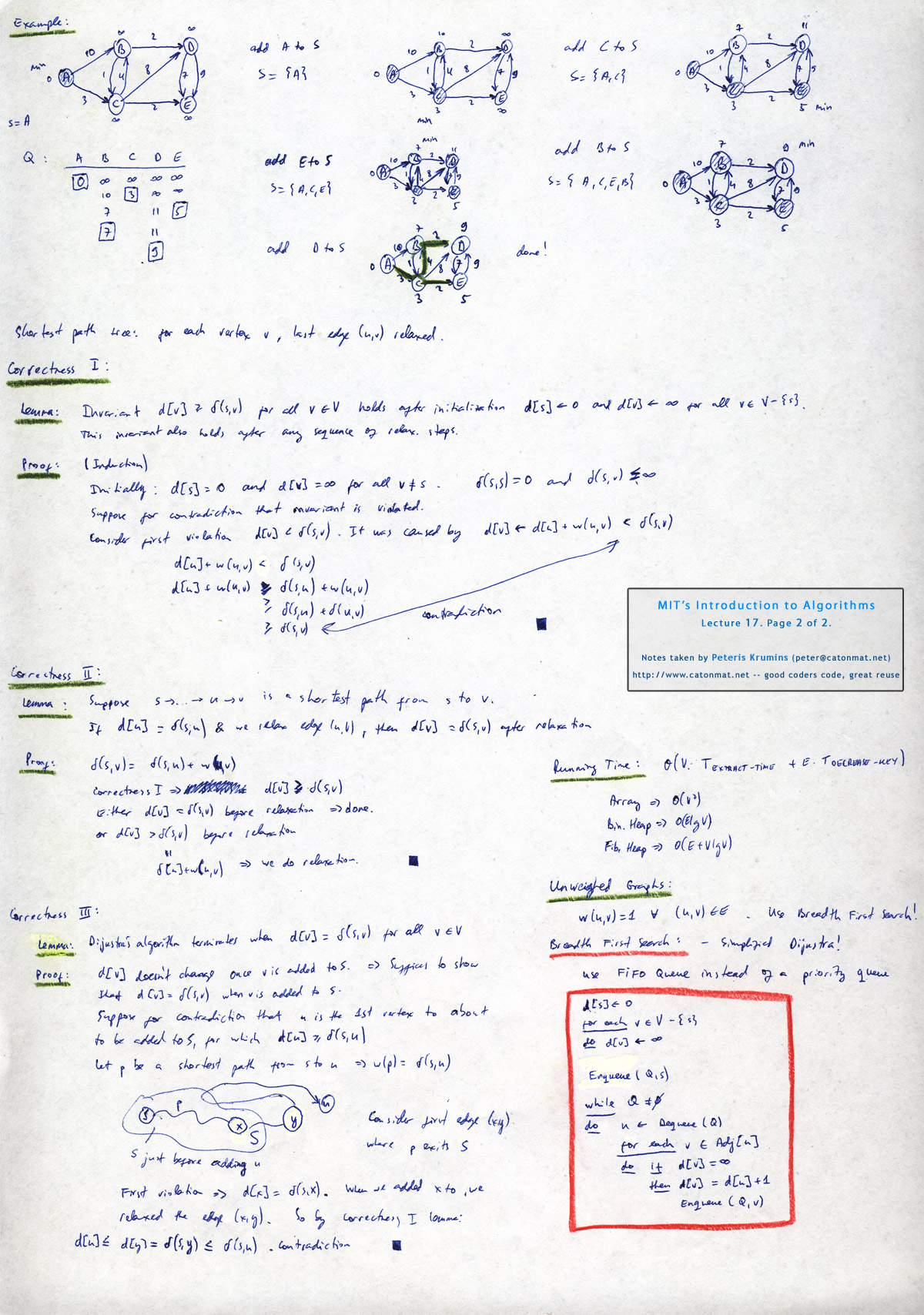
The lecture continues with an example of running Dijkstra's algorithm on a non-trivial graph. It also introduces to a concept of a shortest path tree - a tree that is formed by edges that were last relaxed in each iteration (hard to explain in English, see lecture at 43:40).
The other half of lecture is devoted to three correctness arguments of Dijkstra's algorithm. The first one proves that relaxation never makes a mistake. The second proves that relaxation always makes the right greedy choice. And the third proves that when algorithm terminates the results are correct.
At the final minutes of lecture, running time of Dijkstra's algorithm is analyzed. Turns out that the running time depends on what data structure is used for maintaining the priority queue of the set V-S (step 2). If we use an array, the running time is O(V2), if we use binary heap, it's O(E·lg(V)) and if we use Fibonacci heap, it's O(E + V·lg(V)).
Finally a special case of weighted graphs is considered when all weights are unit weights. In this case a single-source shortest-paths problem can be solved by a the Breadth-first search (BFS) algorithm that is actually a simpler version of Dijkstra's algorithm with priority queue replaced by a FIFO! The running time of BFS is O(V+E).
You're welcome to watch lecture seventeen:
Topics covered in lecture seventeen:
- [01:40] Review of paths.
- [03:15] Edge weight functions.
- [03:30] Example of a path, its edge weights, and weight of the path.
- [04:22] Review of shortest-paths.
- [05:15] Shortest-path weight.
- [06:30] Negative edge weights.
- [10:55] Optimal substructure of a shortest path.
- [11:50] Proof of optimal substructure property: cut and paste.
- [14:23] Triangle inequality.
- [15:15] Geometric proof of triangle inequality.
- [16:30] Single-source shortest paths problem.
- [18:32] Restricted single-source shortest paths problem: all edge weights positive or zero.
- [19:35] Greedy idea for ss shortest paths.
- [26:40] Dijkstra's algorithm.
- [35:30] Example of Dijkstra's algorithm.
- [43:40] Shortest path trees.
- [45:12] Correctness of Dijkstra's algorithm: why relaxation never makes mistake.
- [53:55] Correctness of Dijkstra's algorithm: why relaxation makes progress.
- [01:01:00] Correctness of Dijkstra's algorithm: why it gives correct answer when it terminates.
- [01:15:40] Running time of Dijkstra's algorithm.
- [01:18:40] Running time depending on using array O(V^2), binary heap O(E·lg(V)) and Fibonacci heap O(E + V·lg(V)) for priority queue.
- [01:20:00] Unweighted graphs.
- [01:20:40] Breadth-First Search (BFS) algorithm.
- [01:23:23] Running time of BFS: O(V+E).
Lecture seventeen notes:
 Lecture 17, page 1 of 2: paths, shortest paths, negative edge weights, optimal substructure, triangle inequality, single-source shortest paths, dijkstra's algorithm.
|
 Lecture 17, page 2 of 2: example of dijkstra's algorithm, correctness of dijkstra's algorithm, running time of dijkstra, unweighted graphs, breadth first search (bfs).
|
Lecture 18: Shortest Paths II: Bellman-Ford Algorithm
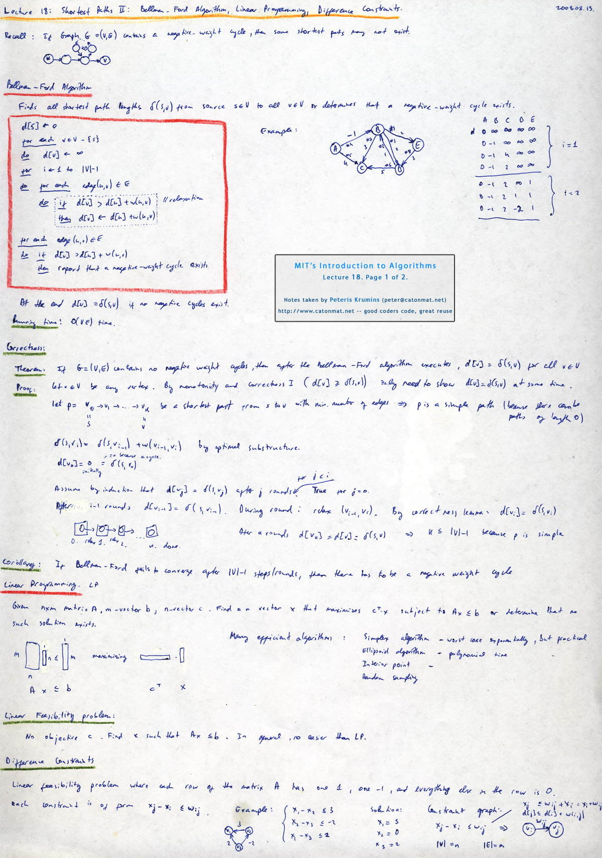
Lecture eighteen begins with recalling that if a graph contains a negative weight cycle, then a shortest path may not exist and gives a geometric illustration of this fact.
Right after this fact, it jumps to Bellman-Ford algorithm. The Bellman-Ford algorithm solves the single-source shortest-paths problem in the general case in which edge weights may be negative. Given a weighted, directed graph G = (V, E) with source s and weight function w: E ? R, the Bellman-Ford algorithm produces the shortest paths from s and their weights, if there is no negative weight cycle, and it produces no answer if there is a negative weight cycle.
The algorithm uses relaxation, progressively decreasing an estimate on the weight of a shortest path from the source s to each vertex v ? V until it achieves the actual shortest-path weight.
The running time of Bellman-Ford algorithm is O(VE). The lecture also gives a correctness proof of Bellman-Ford algorithm.
The other half of the lecture is devoted to a problem that can be effectively solved by Bellman-Ford. It's called the linear feasibility problem that it is a special case of linear programming (LP) problem, where there is no objective but the constraints are in form xi <= wij. It is noted that Bellman-Ford is actually a simple case of LP problem.
The lecture ends with an application of Bellman-Ford to solving a special case of VLSI layout problem in 1 dimension.
You're welcome to watch lecture eighteen:
Topics covered in lecture eighteen:
- [00:20] A long, long time ago... in a galaxy far, far away...
- [00:40] Quick review of previous lecture - Dijkstra's algorithm, non-negative edge weights.
- [01:40] Description of Bellman-Ford algorithm.
- [04:30] Bellman-Ford algorithm.
- [08:50] Running time of Bellman-Ford O(VE).
- [10:05] Example of Bellmen-Ford algorithm.
- [18:40] Correctness of Bellman-Ford algorithm:
- [36:30] Linear programming (LP).
- [42:48] Efficient algorithms for solving LPs: simplex algorithm (exponential in worst case, but practical), ellipsoid algorithm (polynomial time, impractical), interior point methods (polynomial), random sampling (brand new, discovered at MIT).
- [45:58] Linear feasibility problem - LP with no objective.
- [47:30] Difference constraints - constraints in form xj - xi <= wij.
- [49:50] Example of difference constraints.
- [51:04] Constraint graph.
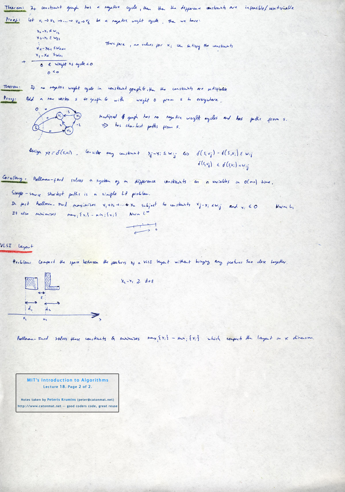
- [54:05] Theorem: Negative weight cycle in constraint means difference constraints are infeasible/unsatisfiable.
- [54:50] Proof.
- [59:15] Theorem: If no negative weight cycle then satisfiable.
- [01:00:23] Proof.
- [01:08:20] Corollary: Bellman-Ford solves a system of of m difference constraints on n variables in O(mn) time.
- [01:12:30] VLSI Layout problem solved by Bellman-Ford.
Lecture eighteen notes:
 Lecture 18, page 1 of 2: bellman-ford algorithm, correctness of bellman-ford, linear programming.
|
 Lecture 18, page 2 of 2: feasibility problem, bellman-ford and difference constraints, vlsi layouts.
|
Lecture 19: Shortest Paths III: All-Pairs Shortest Paths and Floyd-Warshall Algorithm
Lecture nineteen starts with a quick review of lectures seventeen and eighteen. It reminds the running times of various single-source shortest path algorithms, and mentions that in case of a directed acyclic graphs (which was not covered in previous lectures), you can run topological sort and 1 round of Bellman-Ford that makes it find single-source shortest paths in linear time (for graphs) in O(V+E).
The lecture continues all-pairs shortest paths problem, where we want to know the shortest path between every pair of vertices.
A naive approach to this problem is run single-source shortest path from each vertex. For example, on an unweighted graph we'd run BFS algorithm |V| times that would give O(VE) running time. On a non-negative edge weight graph it would be |V| times Dijkstra's algorithm, giving O(VE + V2lg(V)) time. And in general case we'd run Bellman-Ford |V| times that would make the algorithm run in O(V2E) time.
The lecture continues with a precise definition of all-pairs shortest paths problem: given a directed graph, find an NxN matrix (N = |V|), where each entry aij is the shortest path from vertex i to vertex j.
In general case, if the graph has negative edges and it's dense, the best we can do so far is run Bellman-Ford |V| times. Recalling that E = O(V2) in a dense graph, the running time is O(V2E) = O(V4) - hypercubed in number of vertices = slow.
Lecture then proceeds with a dynamic programming algorithm without knowing if it will be faster or not. It's too complicated to explain here, and I recommend watching lecture at 11:54 to understand it. Turns out this dynamic programming algorithm does not give a performance boost and is still O(V4), but it gives some wicked ideas.
The most wicked idea is to connect matrix multiplication with the dynamic programming recurrence and using repeated squaring to beat O(V4). This craziness gives O(V3lgV) time that is an improvement. Please see 23:40 in the lecture for full explanation.
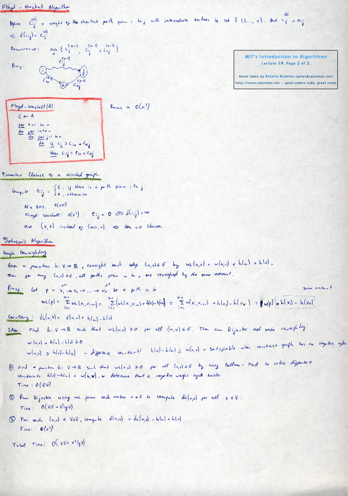
After all this the lecture arrives at Floyd-Warshall algorithm that finds all-pairs shortest paths in O(V3). The algorithm is derived from a recurrence that the shortest path from vertex i to vertex j is minimum of { shortest path from i to j directly or shortest path from i to k and shortest path from k to j }.
Finally the lecture explains Johnson's algorithm that runs in O(VE + V2log(V)) time for sparse graphs. The key idea in this algorithm is to reweigh all edges so that they are all positive, then run Dijkstra from each vertex and finally undo the reweighing.
It turns out, however, that to find the function for reweighing all edges, a set of difference constraints need to be satisfied. It makes us first run Bellman-Ford to solve these constraints.
Reweighing takes O(EV) time, running Dijkstra on each vertex takes O(VE + V2lgV) and undoing reweighing takes O(V2) time. Of these terms O(VE + V2lgV) dominates and defines algorithm's running time (for dense it's still O(V3).
You're welcome to watch lecture nineteen:
Topics covered in lecture nineteen:
- [01:00] Review of single-source shortest path algorithms.
- [04:45] All-pairs shortest paths by running single-source shortest path algorithms from each vertex.
- [05:35] Unweighted edges: |V|xBFS = O(VE).
- [06:35] Nonnegative edge weights: |V|xDijkstra = O(VE + V2lg(V)).
- [07:40] General case: |V|xBellman-Ford = O(V2E).
- [09:10] Formal definition of all-pairs shortest paths problem.
- [11:08] |V|xBellman-Ford for dense graphs (E = O(V2)) is O(V4).
- [11:54] Trying to beat O(V4) with dynamic programming.
- [19:30] Dynamic programming algorithm, still O(V4).
- [23:40] A better algorithm via wicked analogy with matrix multiplication. Running time: O(V3lg(V)).
- [37:45] Floyd-Warshall algorithm. Runs in O(V3).
- [47:35] Transitive closure problem of directed graphs.
- [53:30] Johnson's algorithm. Runs in O(VE + V2log(V))
Lecture nineteen notes:
 Lecture 19, page 1 of 2: all-pairs shortest paths, dynamic programming algorithm, matrix multiplication analogy.
|
 Lecture 19, page 2 of 2: floyd-warshall algorithm, transitive closure problem, johnson's algorithn.
|
This course is taught from the CLRS book, or formally known as Introduction to Algorithms. Chapters 24 and 25, titled Single-Source Shortest Paths and All-Pairs Shortest Paths explain everything I wrote about here in much more detail.
The next post is going to be an introduction to parallel algorithms - things like dynamic multithreading, scheduling and multithreaded algorithms.