 This is the sixth post in an article series about MIT's Linear Algebra course. In this post I will review lecture six on column spaces and null spaces of matrices. The lecture first reviews vector spaces and subspaces and then looks at the result of intersect and union of vector subspaces, and finds out when Ax=b and Ax=0 can be solved.
Here is a list of the previous posts in this article series:
- Lecture 1: Geometry of Linear Equations
- Lecture 2: Elimination with Matrices
- Lecture 3: Matrix Multiplication and Inverse Matrices
- Lecture 4: A=LU Factorization
- Lecture 5: Vector Spaces and Subspaces
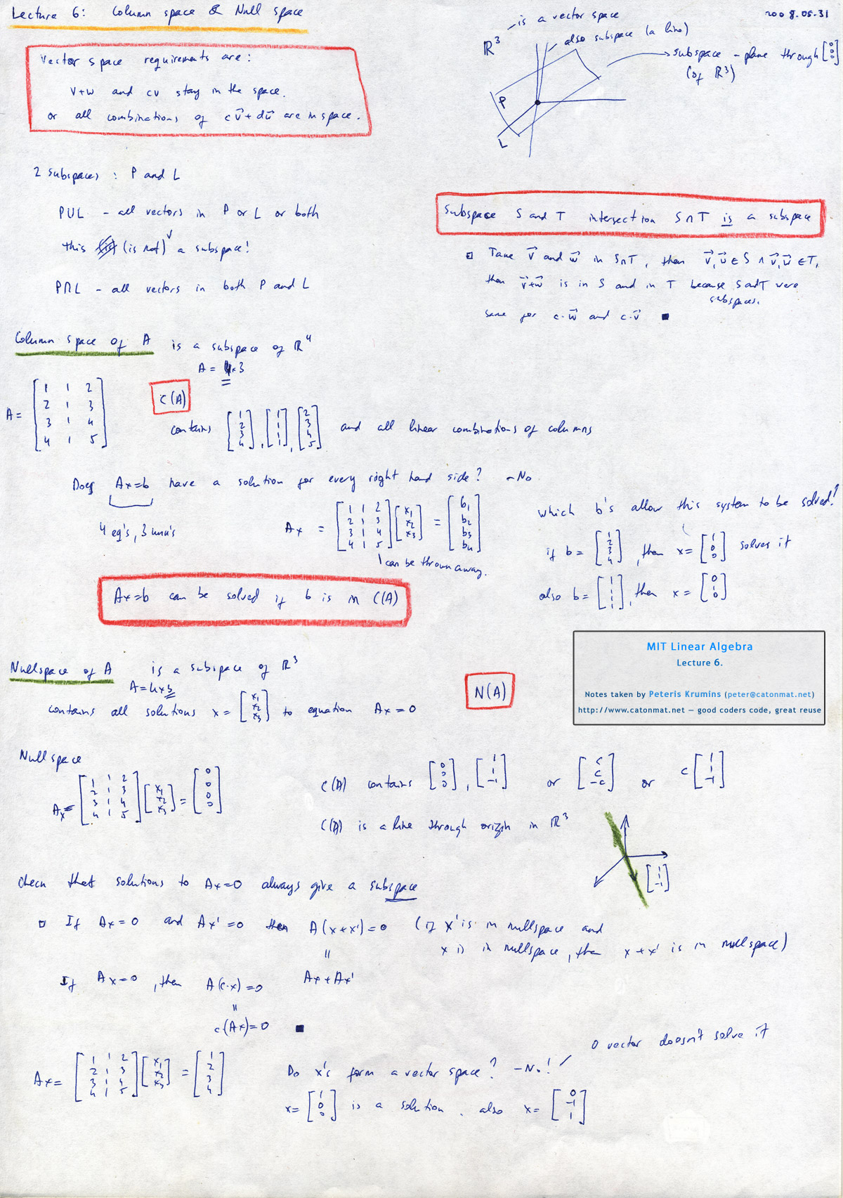
Lecture 6: Column Space and Null Space
Lecture six starts with a reminder of what the vector space requirements are. If vectors v and w are in the space, then the result of adding them and multiplying them by a number stays in the space. In other words, all linear combinations of v and w stay in the space.
For example, the 3-dimensional space R3 is a vector space. You can take any two vectors in it, add them, and multiply them by a number and they will still be in the same R3 space.
Next, the lecture reminds subspaces. A subspace of some space is a set of vectors (including the 0 vector) that satisfies the same two requirements. If vectors v and w are in the subspace, then all linear combinations of v and w are in the subspace.
For example, some subspaces of R3 are:
- Any plane P through the origin (0, 0, 0).
- Any line L through the origin (0, 0, 0).
See the previous, lecture 5, on more examples of spaces on subspaces.
Now suppose we have two subspaces of R3 - plane P and line L. Is the union P?L a subspace? No. Because if we take some vector in P and some vector in L and add them together, we go outside of P and L and that does not satisfy the requirements of a subspace.
What about intersection P?L? Is P?L a subspace? Yes. Because it's either the zero vector or L.
In general, given two subspaces S and T, union S?T is a not a subspace and intersection S?T is a subspace.
The lecture now turns to column spaces of matrices. The notation for a column space of a matrix A is C(A).
For example, given this matrix,
The column space C(A) is all the linear combination of the first (1, 2, 3, 4), the second (1, 1, 1, 1) and the third column (2, 3, 4, 5). That is, C(A) = { a·(1, 2, 3, 4) + b·(1, 1, 1, 1) + c·(2, 3, 4, 5) }. In general, the column space C(A) contains all the linear combinations of columns of A.
A thing to note here is that C(A) is a subspace of R4 because the vectors contain 4 components.
Now the key question, does C(A) fill the whole R4? No. Because there are only three columns (to fill the whole R4 we would need exactly 4 columns) and also because the third column (2, 3, 4, 5) is a sum of first column (1, 2, 3, 4) and second column (1, 1, 1, 1).
From this question follows another question, the most important question in the lecture - Does Ax=b have a solution for every right-hand side vector b? No. Because the columns are not linearly independent (the third can be expressed as first+second)! Therefore the column space C(A) is actually a two-dimensional subspace of R4.
Another important question arises - For which right-hand sides b can this system be solved? The answer is: Ax=b can be solved if and only if b is in the column space C(A)! It's because Ax is a combination of columns of A. If b is not in this combination, then there is simply no way we can express it as a combination.
That's why we are interested in column spaces of matrices. They show when can systems of equation Ax=b be solved.
Now the lecture turns to null spaces of matrices. The notation for a null space of a matrix A is N(A).
Let's keep the same matrix A:
The null space N(A) contains something completely different than C(N). N(A) contains all solutions x's that solve Ax=0. In this example, N(A) is a subspace of R3.
Let's find the null space of A. We need to find all x's that solve Ax=0. The first one, obviously, is x = (0, 0, 0). Another one is x = (1, 1, -1). In general all x's (c, c, -c) solve Ax=0. The vector (c, c, -c) can be rewritten as c·(1, 1, -1).
Note that the null space c·(1, 1, -1) is a line in R3.
The lecture ends with a proof that solutions x to Ax=0 always give a subspace. The first thing to show in the proof is that if x is a solution and x' is a solution, then their sum x + x' is a solution:
We need to show that if Ax=0 and Ax' = 0 then A(x + x') = 0. This is very simple. Matrix multiplication allows to separate A(x + x') into Ax + Ax' = 0. But Ax=0 and Ax'=0. Therefore 0 + 0 = 0.
The second thing to show is that if x is a solution, then c·x is a solution:
We need to show that if Ax=0 then A(c·x)=0. This is again very simple. Matrix multiplication allows to bring c from A(c·x) outside c·A(x) = c·0 = 0.
That's it. We have proven that solutions x to Ax=0 always form a subspace.
Here is the video of the sixth lecture:
Topics covered in lecture six:
- [01:00] Vector space requirements.
- [02:10] Example of spaces R3.
- [02:40] Subspaces of spaces.
- [03:00] A plane P is a subspace of R3.
- [03:50] A line L is a subspace of R3.
- [04:40] Union of P and L.
- [07:30] Intersection of P and L.
- [09:00] Intersection of two subspaces S and T.
- [11:50] The column space C(A) of a matrix A.
- [16:20] Does Ax=b have a solution for every b?
- [19:45] Which b's allow Ax=b to be solved?
- [23:50] Can solve Ax=b exactly when b is in C(A).
- [28:50] The null space N(A) of a matrix A.
- [37:00] Why is the null space a vector space?
- [37:30] A proof that the null space is always a vector space.
- [41:50] Do the solutions to Ax=b form a subspace?
Here are my notes of lecture six:
 My notes of linear algebra lecture 6 on column space and null space.
The next post is going to be about general theory of solving equations Ax=0, pivot variables and special solutions.