 This is going to be my summary of Linear Algebra course from MIT. I watched the lectures of this course in the summer of last year. This was not the first time I'm learning linear algebra. I already read a couple of books and read a few tutorials a couple of years ago but it was not enough for a curious mind like mine.
The reason I am posting these mathematics lectures on my programming blog is because I believe that if you want to be a great programmer and work on the most exciting and world changing problems, then you have to know linear algebra. Larry and Sergey wouldn't have created Google if they didn't know linear algebra. Take a look at this publication if you don't believe me "Linear Algebra Behind Google." Linear algebra has also tens and hundreds of other computational applications, to name a few, data coding and compression, pattern recognition, machine learning, image processing and computer simulations.
The course contains 35 lectures. Each lecture is 40 minutes long, but you can speed them up and watch one in 20 mins. The course is taught by Gilbert Strang. He's the world's leading expert in linear algebra and its applications and has helped the development of Matlab mathematics software. The course is based on working out a lot of examples, there are almost no theorems or proofs.
The textbook used in this course is Introduction to Linear Algebra by Gilbert Strang.
I'll write the summary in the same style as I did my summary of MIT Introduction to Algorithms. I'll split up the whole course in 30 or so posts, each post will contain one or more lectures together with my comments, my scanned notes, embedded video lectures and a timeline of the topics in the lecture. But, not to flood my blog with just mathematics, I will write one or two programming posts in between. You should subscribe to my posts through RSS here.
The whole course is available at MIT's Open Course Ware: Course 18.06, Linear Algebra.
I'll review the first lecture today.
Lecture 1: The Geometry of Linear Equations
The first lecture starts with Gilbert Strang stating the fundamental problem of linear algebra, which is to solve systems of linear equations. He proceeds with an example.
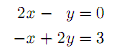
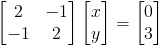
The example is a system of two equations in two unknowns:
There are three ways to look at this system. The first is to look at it a row at a time, the second is to look a column at a time, and the third is use the matrix form.
If we look at this equation a row at a time, we have two independent equations 2x - y = 0 and -x + 2y = 3. These are both line equations. If we plot them we get the row picture:
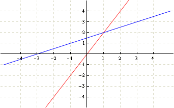
The row picture shows the two lines meeting at a single point (x=1, y=2). That's the solution of the system of equations. If the lines didn't intersect, there would have been no solution.
Now let's look at the columns. The column at the x's is (2, -1), the column at y's is (-1, 2) and the column at right hand side is (0, 3). We can write it down as following:
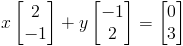
This is a linear combination of columns. What this tells us is that we have to combine the right amount of vector (2, -1) and vector (-1, 2) to produce the vector (0, 3). We can plot the vectors in the column picture:
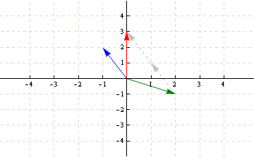
If we take one green x vector and two blue y vectors (in gray), we get the red vector. Therefore the solution is again (x=1, y=2).
The third way to look at this system entirely through matrices and use the matrix form of the equations. The matrix form in general is the following: Ax = b where A is the coefficient matrix, x is the unknown vector and b is the right hand side vector.
How to solve the equations written in matrix form will be discussed in the next lectures. But I can tell you beforehand that the method is called Gauss elimination with back substitution.
For this two equations, two unknowns system, the matrix equation Ax=b looks like this:
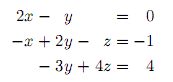
The next example in the lecture is a system of three equations in three unknowns:
We can no longer plot it in two dimensions because there are three unknowns. This is going to be a 3D plot. Since the equations are linear in unknowns x, y, z, we are going to get three planes intersecting at a single point (if there is a solution).
Here is the row picture of 3 equations in 3 unknowns:
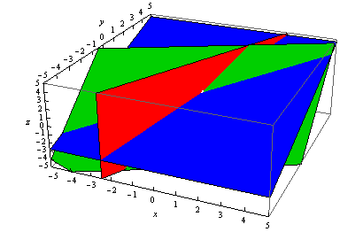
The red is the 2x - y = 0 plane. The green is the -x + 2y - z = -1 plane, and the blue is the -3y + 4z = 4 plane.
Notice how difficult it is to spot the point of intersection? Almost impossible! And all this of going one dimension higher. Imagine what happens if we go 4 or higher dimensions. (The intersection is at (x=0, y=0, z=1) and I marked it with a small white dot.)
The column picture is almost as difficult to understand as the row picture. Here it is for this system of 3 equations in 3 unknowns:
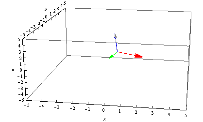
The first column (2, -1, 0) is red, the second column (-1, 2, -3) is green, the fourth column (0, -1, 4) is blue, and the result (0, -1, 4) is gray.
Again, it's pretty hard to visualize how to manipulate these vectors to produce the solution vector (0, -1, 4). But we are lucky in this particular example. Notice that if we take none of red vector, none of green vector and one of blue vector, we get the gray vector! That is, we didn't even need red and green vectors!
This is all still tricky, and gets much more complicated if we go to more equations with more unknowns. Therefore we need better methods for solving systems of equations than drawing plane or column pictures.
The lecture ends with several questions:
- Can Ax = b be solved for any b?
- When do the linear combination of columns fill the whole space?,
- What's the method to solve 9 equations with 9 unknowns?
The examples I analyzed here are also carefully explained in the lecture, you're welcome to watch it:
Topics covered in lecture one:
- [00:20] Information on textbook and course website.
- [01:05] Fundamental problem of linear algebra: solve systems of linear equations.
- [01:15] Nice case: n equations, n unknowns.
- [02:20] Solving 2 equations with 2 unknowns
- [02:54] Coefficient matrix.
- [03:35] Matrix form of the equations. Ax=b.
- [04:20] Row picture of the equations - lines.
- [08:05] Solution (x=1, y=2) from the row picture.
- [08:40] Column picture of the equations - 2 dimensional vectors.
- [09:50] Linear combination of columns.
- [12:00] Solution from the column picture x=1, y=2.
- [12:05] Plotting the columns to produce the solution vector.
- [15:40] Solving 3 equations with 3 unknowns
- [16:46] Matrix form for this 3x3 equation.
- [17:30] Row picture - planes.
- [22:00] Column picture - 3 dim vectors.
- [24:00] Solution (x=0, y=0, z=1) from the column picture by noticing that z vector is equal to b vector.
- [28:10] Can Ax=b be solved for every b?
- [28:50] Do the linear combinations of columns fill the 3d space?
- [32:30] What if there are 9 equations and 9 unknowns?
- [36:00] How to multiply a matrix by a vector? Two ways.
- [36:40] Ax is a linear combination of columns of A.
Here are my notes of lecture one. Sorry about the handwriting. It seems that I hadn't written much at that time and the handwriting had gotten really bad. But it gets better with each new lecture. At lecture 5 and 6 it will be as good as it gets.
 Notes of Linear Algebra lecture 1 on The Geometry of Linear Equations.
The next post is going to be about a systematic way to find a solution to a system of equations called elimination.