![]() This is the thirteenth post in an article series about MIT's lecture course "Introduction to Algorithms." In this post I will review lectures twenty and twenty-one on parallel algorithms. These lectures cover the basics of multithreaded programming and multithreaded algorithms.
This is the thirteenth post in an article series about MIT's lecture course "Introduction to Algorithms." In this post I will review lectures twenty and twenty-one on parallel algorithms. These lectures cover the basics of multithreaded programming and multithreaded algorithms.
Lecture twenty begins with a good overview of multithreaded programming paradigm, introduces to various concepts of parallel programming and at the end talks about the Cilk programming language.
Lecture twenty-one implements several multithreaded algorithms, such as nxn matrix addition, nxn matrix multiplication, and parallel merge-sort. It then goes into great detail to analyze the running time and parallelism of these algorithms.
Lecture 20: Parallel Algorithms I
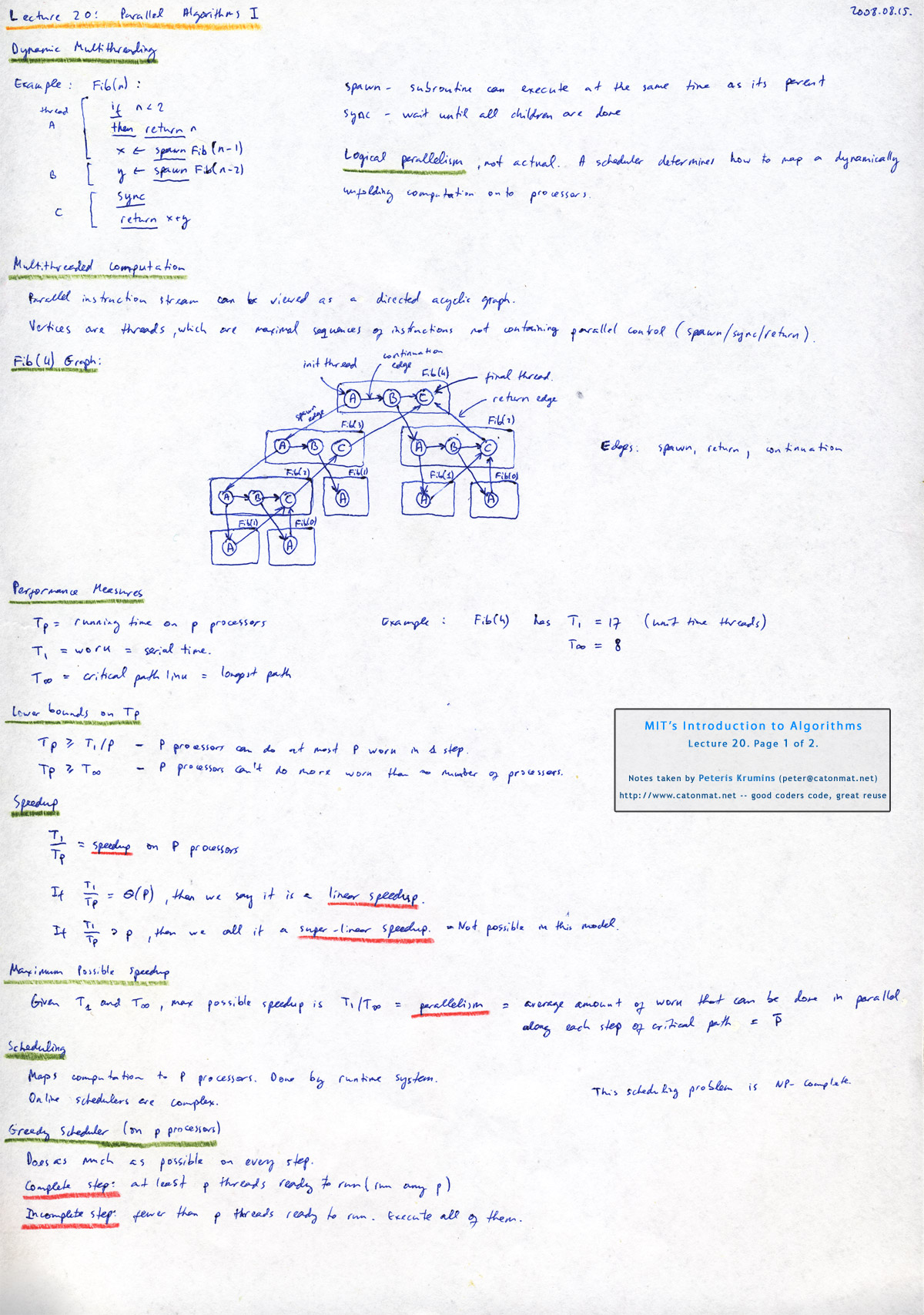
The lecture starts with an introduction to a particular model of parallel computation called dynamic multithreading. It's easiest to understand this model with an example. Here is a multithreaded algorithm that computes Fibonacci numbers:
Fibonacci(n):
1   if n < 2:                     | thread A
2     return n                    | thread A
3   x = <strong>spawn</strong> Fibonacci(n-1)      | thread A
4   y = <strong>spawn</strong> Fibonacci(n-2)      | thread B
5   <strong>sync</strong>                          | thread C
6   return x + y                  | thread C

# this is a really bad algorithm, because it's
# exponential time.
#
# see <a href="https://catonmat.net/mit-introduction-to-algorithms-part-two">lecture three</a> for four different
# classical algorithms that compute Fibonacci numbers
(A thread is defined to be a maximal sequence of instructions not containing the parallel control statements spawn, sync, and return, not something like Java threads or Posix threads.)
I put the most important keywords in bold. They are "spawn" and "sync".
The keyword spawn is the parallel analog of an ordinary subroutine call. Spawn before the subroutine call in line 3 indicates that the subprocedure Fibonacci(n-1) can execute in parallel with the procedure Fibonacci(n) itself. Unlike an ordinary function call, where the parent is not resumed until after its child returns, in the case of a spawn, the parent can continue to execute in parallel with the child. In this case, the parent goes on to spawn Fibonacci(n-2). In general, the parent can continue to spawn off children, producing a high degree of parallelism.
A procedure cannot safely use the return values of the children it has spawned until it executes a sync statement. If any of its children have not completed when it executes a sync, the procedure suspends and does not resume until all of its children have completed. When all of its children return, execution of the procedure resumes at the point immediately following the sync statement. In the Fibonacci example, the sync statement in line 5 is required before the return statement in line 6 to avoid the anomaly that would occur if x and y were summed before each had been computed.
The spawn and sync keywords specify logical parallelism, not "actual" parallelism. That is, these keywords indicate which code may possibly execute in parallel, but what actually runs in parallel is determined by a scheduler, which maps the dynamically unfolding computation onto the available processors.
The lecture then continues with a discussion on how a parallel instruction stream can be viewed as a directed acyclic graph G = (V, E), where threads make up the set V of vertices, and each spawn and return statement makes up an edge in E. There are also continuation edges in E that exist between statements.
In Fibonacci example there are three threads: lines 1, 2, 3 make up the thread A, line 4 is thread B and lines 5, 6 are thread C.
Here is how a graph of Fibonacci(4) computation looks like:
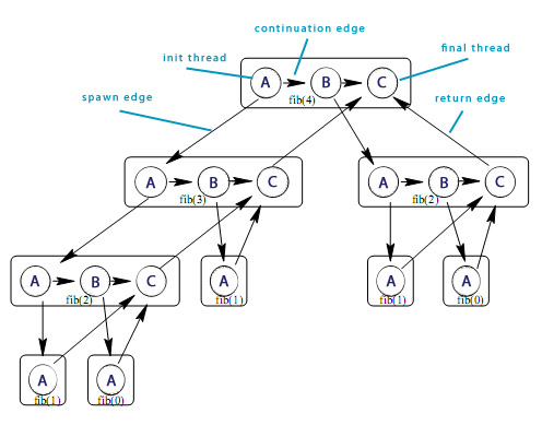 A dag representing multithreaded computation of Fibonacci(4).
Here the threads are show as circles, and each group of threads belonging to the same procedure are surrounded by a rounded rectangle. Downward edges are spawn dependencies, horizontal edges represent continuation dependencies within a procedure, and upward edges are return dependencies. Every computation starts with a single initial thread, and ends with a single final thread.
So to compute Fib(4), first Fib(3) and Fib(2) have to be computed. Fib(4) spawns one thread to compute Fib(3) and another thread to compute Fib(2) and sync'es. In order to compute Fib(3), values of Fib(2) and Fib(1) have to be known, and to compute Fib(2) values of Fib(1) and Fib(0) have to be known. Fib(3) and Fib(2) spawn their threads and sync. This way the computation unwinds.
Next, the lecture introduces some concepts for measuring performance of multithreaded algorithms.
First some time measures:
- Tp - running time of an algorithm on p processors,
- T1 - running time of algorithm on 1 processor, and
- T? as critical path length, that is the longest time to execute the algorithm on infinite number of processors.
Based on these measures, the speedup of a computation on p processors is T1/Tp, that is how much faster a p processor machine executes the algorithm than a one processor machine. If the speedup is O(p), then we say that the computation has a linear speedup. If, however, speedup > p, then we call it a super-linear speedup. The maximum possible speedup is called parallelism and is computed by T1/T?.
After these concepts the lecture puts forward the concept of scheduling and greedy scheduler.
A scheduler maps computation to p processors.
The greedy scheduler schedules as much as it can at every time step. On a p-processor machine every step can be classified into two types. If there are p or more threads ready to execute, the scheduler executes any p of them (this step is also called a complete step). If there are fewer than p threads, it executes all of them (called incomplete step). The greedy scheduler is an offline scheduler and it's 2-competitive (see lecture 13 on online/offline algorithms and the meaning of competitive algorithm).
The lecture ends with an introduction to Cilk parallel, multithreaded programming language. It uses a randomized online scheduler. It was used to write two chess programs *Socrates and Cilkchess.
See Charles Leiseron's handout for a much more comprehensive overview of dynamic multithreading: A Minicourse on Dynamic Multithreaded Algorithms (pdf).
You're welcome to watch lecture twenty:
Topics covered in lecture twenty:
- [01:33] Parallel algorithms.
- [02:33] Dynamic multi-threading.
- [03:15] A multithreaded algorithm for fibonnaci numbers.
- [04:50] Explanation of spawn and sync.
- [06:45] Logical parallelism.
- [08:00] Multithreaded computation.
- [12:15] Fibonacci(4) computation graph, and its concepts - init thread, spawn edge, continuation edge, return edge, final thread.
- [17:45] Edges: spawn, return, continuation.
- [19:40] Performance measures: running time on p processors Tp, work (serial time) T1, critcial path length (longest path) Tinfinity.
- [24:15] Lower bounds on Tp (running time on p processors).
- [29:35] Speedup, linear speedup, superlinear speedup.
- [32:55] Maximum possible speedup.
- [36:40] Scheduling.
- [38:55] Greedy scheduler.
- [43:40] Theorem by Grant and Brent (bound on Tp for greedy scheduler).
- [46:20] Proof of Grant, Brent theorem.
- [56:50] Corollary on greedy scheduler's linear speedup.
- [01:02:20] Cilk programming language.
- [01:06:00] Chess programs: *Socrates, Clikchess.
- [01:06:30] Analysis of *Socrates running time on 512 processors.
Lecture twenty notes:
 Lecture 20, page 1 of 2: dynamic multithreading, multithreaded computation, performance measures, speedup, scheduling, greedy scheduler.
|
 Lecture 20, page 2 of 2: grant, brent theorem, cilk, socrates, cilkchess.
|
Lecture 21: Parallel Algorithms II
Lecture twenty-one is all about real multithreaded algorithms and their analysis.
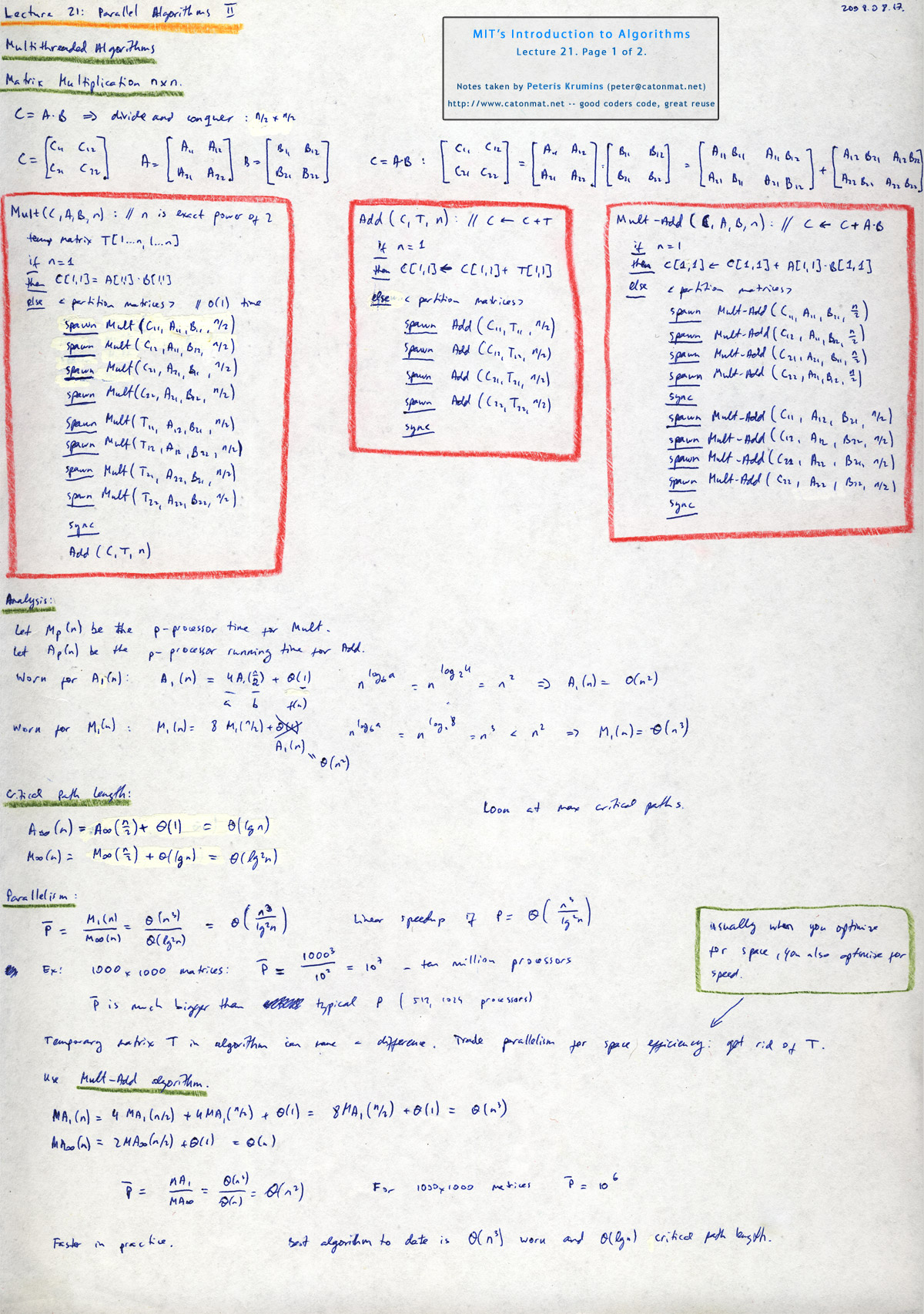
It starts with a hugly important problem of multithreaded matrix multiplication: given two nxn matrices A and B, write a multithreaded algorithm Matrix-Multiply that multiplies them, producing matrix C. The natural approach is to use divide and conquer method from lecture three, and formulate the problem as follows:
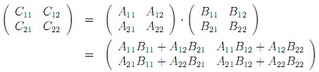
Each nxn matrix can be expressed as 8 multiplications and 4 additions of (n/2)x(n/2) submatrices. So the first thing we need is Matrix-Add algorithm that adds two matrices in parallel.
Here is the parallel Matrix-Add algorithm:
Matrix-Add(C, T, n):
   // Adds matrices C and T in-place, producing C = C + T
   // n is power of 2 (for simplicity).
   if  n == 1:
     C[1, 1] = C[1, 1] + T[1, 1]
   else:
     partition C and T into (n/2)<small>x</small>(n/2) submatrices
     spawn Matrix-Add(C<sub>11</sub>, T<sub>11</sub>, n/2)
     spawn Matrix-Add(C<sub>12</sub>, T<sub>12</sub>, n/2)
     spawn Matrix-Add(C<sub>21</sub>, T<sub>21</sub>, n/2)
     spawn Matrix-Add(C<sub>22</sub>, T<sub>22</sub>, n/2)
     sync
The base case for this algorithm is when matrices are just scalars, then it just adds the only element of both matrices. In all other cases, it partitions matrices C and T into (n/2)x(n/2) matrices and spawns four subproblems.
Now we can implement the Matrix-Multiply algorithm, by doing 8 multiplications in parallel and then calling Matrix-Add to do 4 additions.
Here is the parallel Matrix-Multiply algorithm:
Matrix-Multiply(C, A, B, n):
   // Multiplies matrices A and B, storing the result in C.
   // n is power of 2 (for simplicity).
   if  n == 1:
     C[1, 1] = A[1, 1] · B[1, 1]
   else:
     allocate a temporary matrix T[1...n, 1...n]
     partition A, B, C, and T into (n/2)<small>x</small>(n/2) submatrices
     spawn Matrix-Multiply(C<sub>12</sub>,A<sub>11</sub>,B<sub>12</sub>, n/2)
     spawn Matrix-Multiply(C<sub>21</sub>,A<sub>21</sub>,B<sub>11</sub>, n/2)
     spawn Matrix-Multiply(C<sub>22</sub>,A<sub>21</sub>,B<sub>12</sub>, n/2)
     spawn Matrix-Multiply(T<sub>11</sub>,A<sub>12</sub>,B<sub>21</sub>, n/2)
     spawn Matrix-Multiply(T<sub>12</sub>,A<sub>12</sub>,B<sub>22</sub>, n/2)
     spawn Matrix-Multiply(T<sub>21</sub>,A<sub>22</sub>,B<sub>21</sub>, n/2)
     spawn Matrix-Multiply(T<sub>22</sub>,A<sub>22</sub>,B<sub>22</sub>, n/2)
     sync
     Matrix-Add(C, T, n)
The lecture then proceeds to calculating how good the algorithm is, turns out the parallelism (ratio of time of algorithm running on a single processor T1 to running on infinite number of processors Tinf) for doing 1000x1000 matrix multiplication is 107, which the parallel algorithm is fast as hell.
Matrix-Multiply used a temporary matrix which was actually unnecessary. To achieve higher performance, it's often advantageous for an algorithm to use less space, because more space means more time. Therefore a faster algorithm can be added that multiplies matrices and adds them in-place. See lecture at 33:05 for Matrix-Multiply-Add algorithm. The parallelism of this algorithm for 1000x1000 matrix multiplication is 106, smaller than the previous one, but due to fact that no temporary matrices had to be used, it beats Matrix-Multiply algorithm in practice.
The lecture then proceeds to parallel sorting. The classical sorting algorithms were covered in lectures four and five. This lecture parallelizes the Merge-Sort algorithm.
Here is the parallel merge-sort algorithm:
Parallel-Merge-Sort(A, p, r): // sort A[p...r]
  if p < r:
    q = floor((p+r)/2)
    spawn Parallel-Merge-Sort(A, p, q)
    spawn Parallel-Merge-Sort(A, q+1, r)
    sync
    Merge(A, p, q, r) // merge A[p...q] with A[q+1...r]
Instead of recursively calling Parallel-Merge-Sort for subproblems, we spawn them, thus utilizing the power of parallelism. After doing analysis turns out that due to fact that we use the classical Merge() function, the parallelism is just lg(n). That's puny!
To solve this problem, a Parallel-Merge algorithm has to be written. The lecture continues with presenting a Parallel-Merge algorithm, and after that does the analysis of the same Parallel-Merge-Sort algorithm but with Parallel-Merge function. Turns out this algorithm has parallelism of n/lg2(n), that is much better. See lecture at 51:00 for Parallel-Merge algorithm.
The best parallel sorting algorithm know to date has the parallelism of n/lg(n).
You're welcome to watch lecture twenty-one:
Topics covered in lecture twenty-one:
- [00:35] Multithreaded algorithms.
- [01:32] Multithreaded matrix multiplication.
- [02:05] Parallelizing with divide and conquer.
- [04:30] Algorithm Matrix-Multiply, that computes C = A*B.
- [10:13] Algorithm Matrix-Add, that computes C = C+T.
- [12:45] Analysis of running time of Matrix-Multiply and Matrix-Add.
- [19:40] Analysis of critical path length of Matrix-Multiply and Matrix-Add.
- [26:10] Parallelism of Matrix-Multiply and Matrix-Add.
- [33:05] Algorithm Matrix-Multiply-Add, that computes C = C + A*B.
- [35:50] Analysis of Matrix-Multiply-Add.
- [42:30] Multithreaded, parallel sorting.
- [43:30] Parallelized Merge-Sort algorithm.
- [45:55] Analysis of multithreaded Merge-Sort.
- [51:00] Parallel-Merge algorithm.
- [01:00:30] Analysis of Parallel-Merge algorithm.
Lecture twenty-one notes:
 Lecture 21, page 1 of 2: multithreaded algorithms, matrix multiplication, analysis (critical path length, parallelism).
|
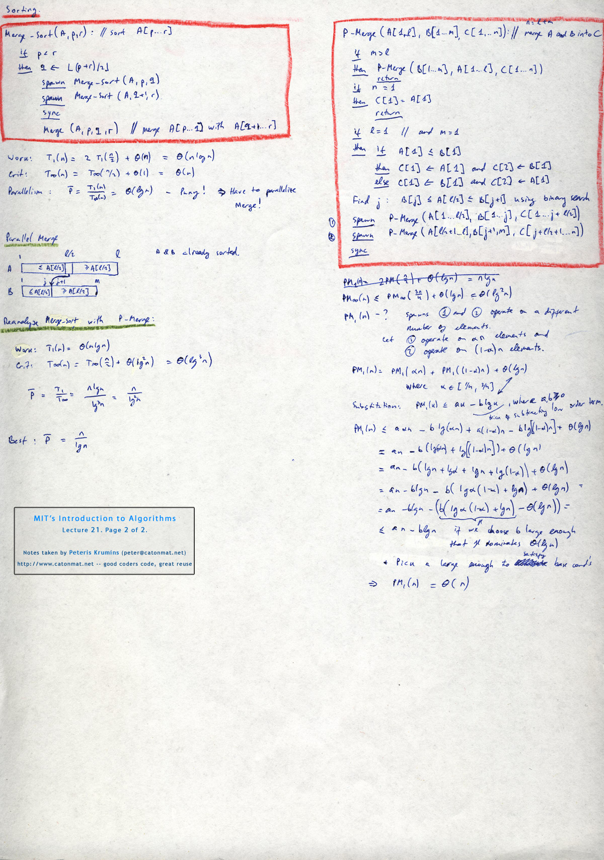 Lecture 21, page 2 of 2: paralel sorting, merge sort, parallel merge, analysis.
|
Have fun with parallel, multithreaded algorithms! The next post is going to be on cache oblivious algorithms! They are a class of algorithms that exploit all the various caches in modern computer architecture to make them run notably faster.